A Deep Dive into Transformers with TensorFlow and Keras: Part 1

---

Table of Contents

---

A Deep Dive into Transformers with TensorFlow and Keras: Part 1

While we look at gorgeous futuristic landscapes generated by AI or use massive models to write our own tweets, it is important to remember where all this started.

Data, matrix multiplications, repeated and scaled with non-linear switches. Maybe that simplifies things a lot, but even today, most architectures boil down to these principles. Even the most complex systems, ideas, and papers can be boiled down to just that:

Data, matrix multiplications, repeated and scaled with non-linear switches.

Over the past few months, we have covered Natural Language Processing (NLP) through our tutorials. We started from the very history and foundation of NLP and discussed Neural Machine Translation with attention.

Here are all the tutorials chronologically.

• Introduction to Natural Language Processing (NLP)
• Introduction to the Bag-of-Words (BoW) Model
• Word2Vec: A Study of Embeddings NLP
• Comparison Between BagofWords and Word2Vec
• Introduction to Recurrent Neural Networks with Keras and TensorFlow
• Long Short-Term Memory Networks
• Neural Machine Translation
• Neural Machine Translation with Bahdanau’s Attention Using TensorFlow and Keras
• Neural Machine Translation with Luong’s Attention Using TensorFlow and Keras

Now, the progression of NLP, as discussed, tells a story. We begin with tokens and then build representations of these tokens. We use these representations to find similarities between tokens and embed them in a high-dimensional space. The same embeddings are also passed into sequential models that can process sequential data. Those models are used to build context and, through an ingenious way, attend to parts of the input sentence that are useful to the output sentence in translation.

Phew! That was a lot of research. We are almost something of a scientist ourselves.

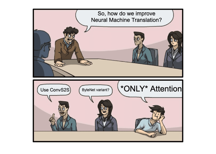
But what lies ahead? A group of real scientists got together to answer that question and formulate a genius plan (as shown in Figure 1) that would shake the field of Deep Learning to its very core.

In this tutorial, you will learn about the evolution of the attention mechanism that led to the seminal architecture of Transformers.

This lesson is the 1st in a 3-part series on NLP 104:

1. A Deep Dive into Transformers with TensorFlow and Keras: Part 1 (today’s tutorial)
2. A Deep Dive into Transformers with TensorFlow and Keras: Part 2
3. A Deep Dive into Transformers with TensorFlow and Keras: Part 3

To learn how the attention mechanism evolved into the Transformer architecture, just keep reading.

---

A Deep Dive into Transformers with TensorFlow and Keras: Part 1

---

Introduction

In our previous blog post, we covered Neural Machine Translation models based on Recurrent Neural Network architectures that include an encoder and a decoder. In addition, to facilitate better learning, we also introduce the attention module.

Vaswani et al. proposed a simple yet effective change to the Neural Machine Translation models. An excerpt from the paper best describes their proposal.

We propose a new simple network architecture, the Transformer, based solely on attention mechanisms, dispensing with recurrence and convolutions entirely.

In today’s tutorial, we will cover the theory behind this neural network architecture called the Transformer. We will focus on the following in this tutorial:

• The Transformer Architecture
  • Encoder
  • Decoder
• Evolution of Attention
  • Version 0
  • Version 1
  • Version 2
  • Version 3
  • Version 4 (Cross-Attention)
  • Version 5 (Self-Attention)
  • Version 6 (Multi-Head Attention)

---

The Transformer Architecture

We take a top-down approach in building the intuitions behind the Transformer architecture. Let us first look at the entire architecture and break down individual components later.

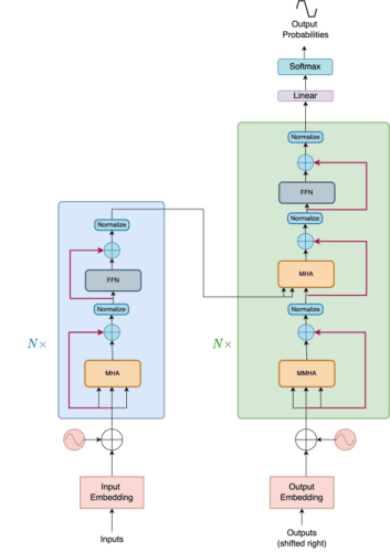
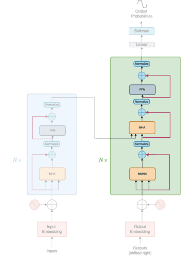
The Transformer consists of two individual modules, namely the Encoder and the Decoder, as shown in Figure 2.

---

Encoder

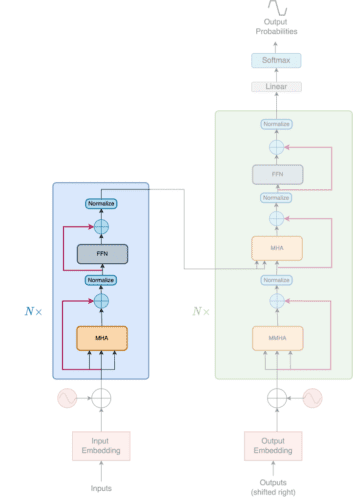
As shown in Figure 3, the encoder is a stack of identical layers. Each layer is composed of two sub-layers.

The first is a multi-head self-attention mechanism, and the second is a simple, position-wise, fully connected feed-forward network.

The authors also employ residual connections (red lines) and a normalization operation around the two sub-layers.

The source tokens are first embedded into a high-dimensional space. The input embeddings are added with positional encoding (we will cover positional encodings in depth later in the tutorial series). The summed embeddings are then fed into the encoder.

---

Decoder

As shown in Figure 4, the decoder is a stack of identical layers. Each layer is composed of three sub-layers.

In addition to the two sub-layers in each encoder layer, the decoder inserts a third sub-layer, which performs multi-head attention over the output of the encoder stack.

The decoder also has residual connections and a normalization operation around the three sub-layers.

Notice that the first sublayer of the decoder is a masked multi-head attention layer instead of a multi-head attention layer.

The target tokens are offset by one. Like the encoder, the tokens are first embedded into a high-dimensional space. The embeddings are then added with positional encodings. The summed embeddings are then fed into the decoder.

This masking, combined with the fact that the target tokens are offset by one position, ensures that the predictions for position can depend only on the known outputs at positions less than .

---

Evolution of Attention

The encoder and decoder have been built around a central piece called the Multi-Head Attention module. This piece of the architecture is the formula X that has placed Transformers at the top of the Deep Learning food chain. But Multi-Head Attention (MHA) did not always exist in its present form.

We have studied a very basic form of attention in the prior blog posts covering the Bahdanau and Luong attentions. However, the journey from the early form of attention to the one that is actually used in the Transformers architecture is long and full of monstrous notations.

But do not fear. Our quest will be to navigate the different versions of attention and counter any problems we might face. At the end of our journey, we shall emerge with an intuitive understanding of how attention works in the Transformer architecture.

---

Version 0

To understand the intuition of attention, we start with an input and a query. Then, we attend to parts of the input based on the query. So if you have an image of a landscape and someone asks you to decipher the weather there, you would attend to the sky first. The image is the input, while the query is “how is the weather there?”

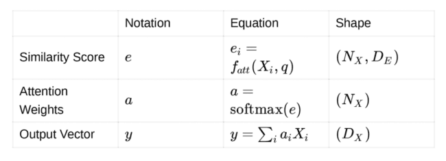
In terms of computation, attention is given to parts of the input matrix which is similar to the query vector. We compute the similarity between the input matrix and the query vector. After we obtain the similarity score, we transform the input matrix into an output vector. The output vector is the weighted summation (or average) of the input matrix.

Intuitively the weighted summation (or average) should be richer in representation than the original input matrix. It includes the “where and what to attend to.” The diagram of this baseline version (version 0) is shown in Figure 5.

Inputs:

Similarity function: , which is a **feed-forward network**. The feed-forward network takes the query and input, and projects both of them to dimension .

Outputs:

---

Version 1

The two most commonly used attention functions are additive attention and dot-product (multiplicative) attention. Additive attention computes the compatibility function using a feed-forward network.

The first change we make to the mechanism is swapping out the feed-forward network with a dot product operation. Turns out that this is highly efficient with reasonably good results. While we use the dot product, notice how the shape of the input vectors now changes to incorporate the dot product. The diagram of version 1 is shown in Figure 6.

Inputs:

Similarity function: Dot Product

Outputs:

---

Version 2

In this section, we will discuss a very important concept realized in the paper. The authors propose “scaled dot product” instead of “normal dot product” as the similarity function. The scaled dot product is exactly the same as the dot product, but scaled with a factor of .

Here let us pose some problems and devise the solutions ourselves. The scaling factor will be hidden inside the solution.

---

Problems

• Vanishing Gradient Problem: The weights of a Neural Network update in proportion to the gradient of the loss. The problem is that, in some cases, the gradient will be small, effectively preventing the weight from changing its value at all. This, in turn, prohibits the network from learning any further. This is often referred to as the vanishing gradient problem.
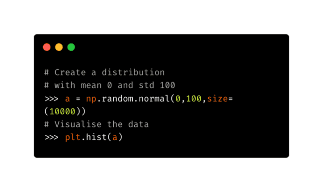
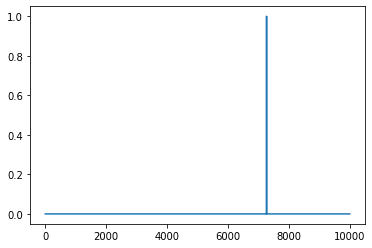
• Unnormalized softmax: Consider a normal distribution. The softmax of the distribution is heavily dependent on its standard deviation. With a huge standard deviation, the softmax will result in a peak with zeros all around. Figures 7-10 help visualize the problem.

• Unnormalized softmax leading to the vanishing gradient: Consider if your logits pass through softmax and then we have a loss (cross-entropy). The errors that backpropagate will be dependent on the softmax output.
  
  Now assume that you have an unnormalized softmax function, as mentioned above. The error corresponding to the peak will definitely be back-propagated, while the others (corresponding to zeros in the softmax) will not flow at all. This gives rise to the vanishing gradient problem.

---

Solution

To counter the problem of vanishing gradients due to unnormalized softmax, we need to find a way to have a better softmax output.

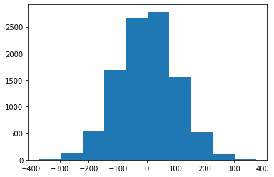
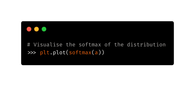
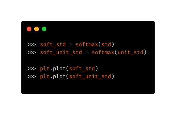
It turns out that the standard deviation of a distribution largely influences the softmax output. Let’s create a normal distribution with a standard deviation of 100. We also scale the distribution so that the standard deviation is unity. The code to create the distribution and scale it can be found in Figure 11. Figure 12 visualizes the histograms of the distributions.

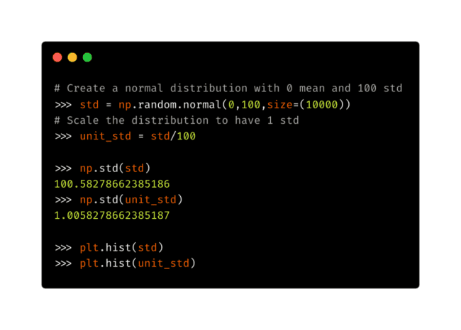
The histograms of both distributions seem alike. One is the scaled version of the other (look at the x-axis).

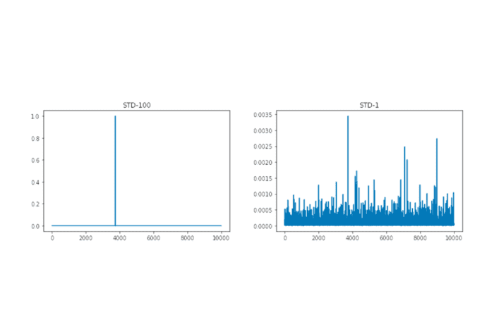
Let’s calculate the softmax of both and visualize them as shown in Figures 13 and 14.

Scaling the distribution to unit standard deviation provides a distributed softmax output. This softmax allows the gradients to backpropagate, saving our model from collapsing.

---

Scaling of the Dot Product

We came across the vanishing gradient problem, the unnormalized softmax output, and also a way we can counter it. We are yet to understand the relationship between the above-mentioned problems and solutions to that of the scaled dot product proposed by the authors.

The attention layers consist of a similarity function that takes two vectors and performs a dot product. This dot product is then passed through a softmax to create the attention weights. This recipe is perfect for a vanishing gradient problem. The way to counter the problem is to transform the dot product result into a unit standard deviation distribution.

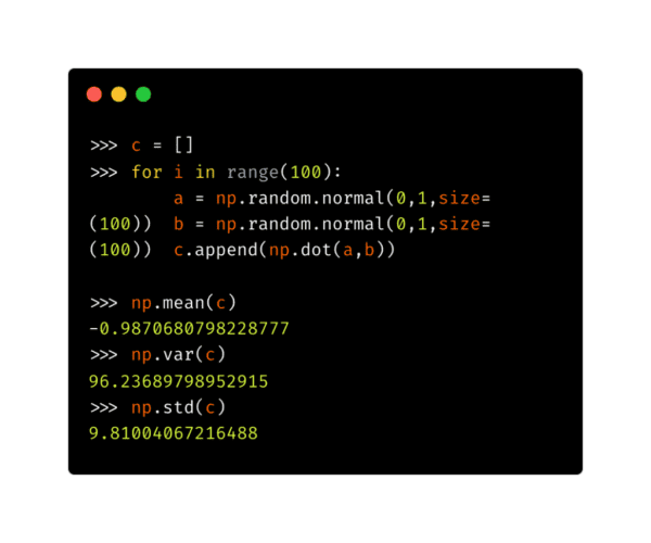
Let us assume that we have two independent and randomly distributed variables: and , as shown in Figure 15. Both vectors have a mean of 0 and a standard deviation of 1.

What is interesting here is that the mean of such a dot product remains to be 0 regardless of the size of the random variables, but the variance and, in turn, the standard deviation are directly proportional to the size of the random variables. To be specific, variance is linearly proportional while standard deviation is proportional with the factor of .

To prohibit the dot product from a vanishing gradient problem, the authors scale the dot product with the factor. This, in turn, is the scaled dot product that the authors have suggested in the paper. The visualization of Version 2 is shown in Figure 16.

Inputs:

Similarity function: Dot Product

Outputs:

---

Version 3

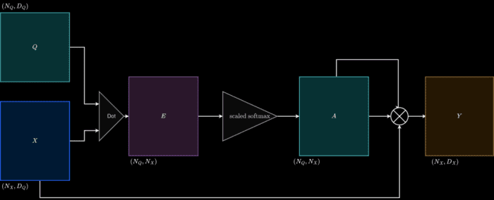
Previously we looked at a single query vector. Let us scale this implementation to multiple query vectors. We calculate the similarities of the input matrix with all the query vectors (query matrix) we have. The visualization of Version 3 is shown in Figure 17.

Inputs:

Similarity function: Dot Product

Outputs:

---

Version 4 (Cross-Attention)

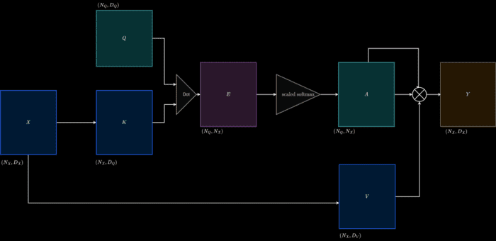
To build cross-attention, we make some changes. The changes are specific to the input matrix. As we already know, attention needs an input matrix and a query matrix. Suppose we projected the input matrix into a pair of matrices, namely the key and value matrices.

The key matrix is attended to with respect to the query matrix. This results in attention weights. Here the value matrix is transformed with the attention weights as opposed to the input matrix transformation, as seen earlier.

This is done to decouple the complexity. The input matrix can now have a better projection that takes care of building attention weights and better output matrices as well. The visualization of Cross Attention is shown in Figure 18.

Inputs:

Similarity function: Dot Product

Outputs:

---

Version 5 (Self-Attention)

With cross-attention, we learned that there are three matrices in the attention module: key, value, and query. The key and value matrix are projected versions of the input matrix. What if the query matrix also was projected from the input?

This results in what we call self-attention. Here the main motivation is to build a richer implementation of self with respect to self. This sounds funny, but it is highly important and forms the basis of the Transformer architecture. The visualization of Self-Attention is shown in Figure 19.

Inputs:

Similarity function: Dot Product

Outputs:

---

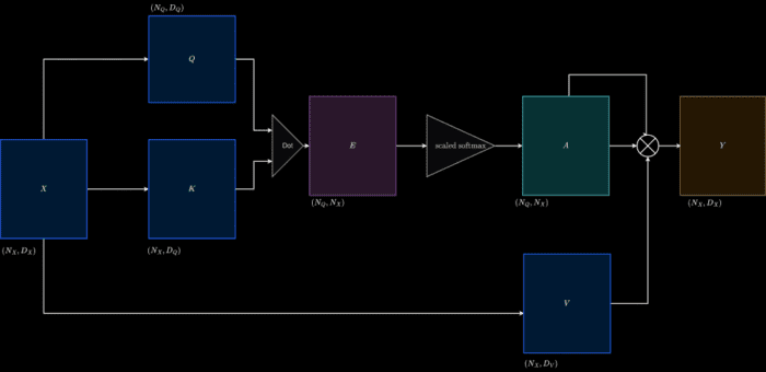
Version 6 (Multi-Head Attention)

This is the last stage of evolution. We have come a long way. We started by building the intuition of attention, and now we will discuss multi-head (self) attention.

The authors wanted to decouple relations further by introducing multiple heads of attention. This means that the key, value, and query matrices are now split into a number of heads and projected. The individual splits are then passed into a (self) attention module (described above).

All the splits are then concatenated into a single representation. The visualization of Multi-Head Attention is shown in Figure 20.

If you have come this far, take a pause and congratulate yourselves. The journey has been long and filled with monstrous notations and numerous matrix multiplications. But as promised, we now have an intuitive sense of how Multi-Head Attention evolved. To recap:

• Version 0 started with the baseline, where the similarity function is computed between an input and a query using a feed-forward network.
• Version 1 saw us swap that feed-forward network for a simple dot product.
• Due to problems like vanishing gradients and unnormalized probability distribution, we use a scaled dot product in Version 2.
• In Version 3, we use multiple query vectors rather than just one.
• In Version 4, we build the cross-attention layer by breaking the input vector into key and value matrices.
• Whatever is found outside can also be found inside. Thus in Version 5, we obtain the query vector from the input as well, calling this the self-attention layer.
• Version 6 is the last and final form, where we see all relations between query, key, and value being further decoupled by using multiple heads.

Transformers might have multiple heads, but we have only one, and if it is spinning right now, we do not blame you. Here is an interactive demo to visually recap whatever we have learned thus far.

---

---

Summary

Attention is all you need, was published in the year 2017. Since then, it has absolutely revolutionized Deep Learning. Almost all tasks and novel architectures have leveraged Transformers as a whole or in parts.

The novelty of the architecture stands out when we study the evolution of the attention mechanism rather than singularly focusing on the version used in the paper.

This tutorial focused on developing this central piece: the Multi-Head Attention layer. In upcoming tutorials, we will learn about the connecting wires (feed-forward layers, positional encoding, and others) that hold the architecture together and also how to code the architecture in TensorFlow and Keras.

---

Citation Information

A. R. Gosthipaty and R. Raha. “A Deep Dive into Transformers with TensorFlow and Keras: Part 1,” PyImageSearch, P. Chugh, S. Huot, K. Kidriavsteva, and A. Thanki, eds., 2022, https://pyimg.co/8kdj1

@incollection{ARG-RR_2022_DDTFK1,
  author = {Aritra Roy Gosthipaty and Ritwik Raha},
  title = {A Deep Dive into Transformers with {TensorFlow} and {K}eras: Part 1},
  booktitle = {PyImageSearch},
  editor = {Puneet Chugh and Susan Huot and Kseniia Kidriavsteva and Abhishek Thanki},
  year = {2022},
  note = {https://pyimg.co/8kdj1},
}

---