Long Short-Term Memory Networks

---

Table of Contents

---

Long Short-Term Memory Networks

In this tutorial, we will learn how to train a movie review sentiment classification model using Long Short-Term Memory (LSTM) Networks introduced by Hochreiter and Schmidhuber. In our previous tutorial, Introduction to Recurrent Neural Networks with Keras and TensorFlow, we were introduced to the task of movie review sentiment classification.

As before, we will use the imdb_reviews, a dataset of 25,000 highly polar movie reviews.

We will also understand some of the shortcomings of Recurrent Neural Networks and how to circumvent them using Long Short-Term Memory Networks.

This lesson is the 2nd in a 3-part series on NLP 102:

1. Introduction to Recurrent Neural Networks with Keras and TensorFlow
2. Long Short-Term Memory Networks (today’s tutorial)
3. Neural Machine Translation

To learn how to build a Long Short-Term Memory Network for sentiment classification using TensorFlow and Keras, just keep reading.

---

Long Short-Term Memory Networks

---

Introduction

At its core, LSTMs are an extension of Recurrent Neural Networks. RNNs are great for modeling sequential data, but they strictly do not have much efficiency in retaining information for a long period.

This means a word at the beginning of a long sentence will lose its context by the end. Not a very useful feature for a language or sequence model.

LSTMs are aimed at solving this problem. Typically as the name suggests, LSTMs aim to retain long-term information from the sequence.

Before we begin this tutorial, it is advisable to go through the previous tutorial in this series to familiarize ourselves with the code and project structure. A number of modules have been reused from the RNN code.

---

Configuring Your Development Environment

To follow this guide, you need to have TensorFlow, TensorFlow Datasets, and the Matplotlib library installed on your system.

Luckily, all are pip-installable:

$ pip install tensorflow
$ pip install tensorflow_datasets
$ pip install matplotlib

---

Having Problems Configuring Your Development Environment?

All that said, are you:

• Short on time?
• Learning on your employer’s administratively locked system?
• Wanting to skip the hassle of fighting with the command line, package managers, and virtual environments?
• Ready to run the code right now on your Windows, macOS, or Linux system?

Then join PyImageSearch University today!

Gain access to Jupyter Notebooks for this tutorial and other PyImageSearch guides that are pre-configured to run on Google Colab’s ecosystem right in your web browser! No installation required.

And best of all, these Jupyter Notebooks will run on Windows, macOS, and Linux!

---

Project Structure

We first need to review our project directory structure.

Start by accessing the “Downloads” section of this tutorial to retrieve the source code and example images.

From there, take a look at the directory structure:

$ tree -dirsfirst
.
|____ output
| |____ lstm_plot.png
| |____ rnn_plot.png
|____ pyimagesearch
| |____ plot.py
| |____ save_load.py
| |____ config.py
| |____ standardization.py
| |____ __init__.py
| |____ model.py
| |____ dataset.py
|____ train.py
|____ inference.py
|____ terminal_output.txt

In the pyimagesearch directory, we have:

• plot.py: Script to help us visualize outputs.
• save_load.py: Script to save and load the trained model weights.
• config.py: Script containing the entire configuration pipeline.
• standardization.py: Script containing utilities to help us prepare the data pipeline.
• __init__.py: Script that turns the directory into a python package.
• model.py: Script housing the model.
• dataset.py: Script to help us load the data to our project.

In the core directory, we have two scripts:

• train.py: Script to train the LSTM model.
• inference.py: Script to draw inference from our trained LSTM model.

Note: The code download for this blog post also contains code snippets for Recurrent Neural Networks (RNNs). These are covered in a previous blog post: Introduction to Recurrent Neural Networks with Keras and TensorFlow.

---

Modeling Sequential Data with RNNs

In the previous tutorial, we modeled sequential data with Recurrent Neural Networks. We learned how the RNN learns from the current input and all the previous hidden states. This is demonstrated in Figure 2.

However, RNNs are not perfect when it comes to modeling sequential data. Certain shortcomings need to be addressed to improve its architecture.

---

The Problem with RNNs

Recurrent Neural Networks have a serious problem, and the problem stems from their strength: the recurrence. To fully appreciate the situation, one needs to look at the gradients and the backpropagation formulae for RNNs.

We begin with the recurrence formula.

Now we take the derivative of the current hidden state with the previous one. Hold on to this equation, as we will need it later.

So to backpropagate in an RNN, we calculate the gradient loss with respect to the weights. Unfortunately, due to recurrence, the chain rule looks a little intimidating.

To condense the terms, we can represent them with a product notation.

Let’s expand equation (3b) using equation (2). Finally, the gradient formula looks like this.

Now that we are done with the equations, let’s drive the point home. In the interactive demo, we plotted three graphs:

• tanh
• derivative of tanh
• product of the derivative term

Do you notice something?

The graph goes closer to zero as the number of product terms increases. Likewise, as the recurrence increases, the derivative term will get closer to zero. In other words, recurrence can lead to the “vanishing gradient.”

Vanishing gradient is notoriously difficult to manage. It is proven to be a bottleneck for RNNs. With gradients vanishing, the weights are seldom optimized, and the network learns poorly.

---

Long Short-Term Memory Networks

In a vanilla RNN, the gradient flow was faulty. As a consequence, the RNN did not learn a longer context. With LSTMs, we want to counter the problem. The architecture of Long Short-Term Memory Networks provides a better way for the gradients to backpropagate.

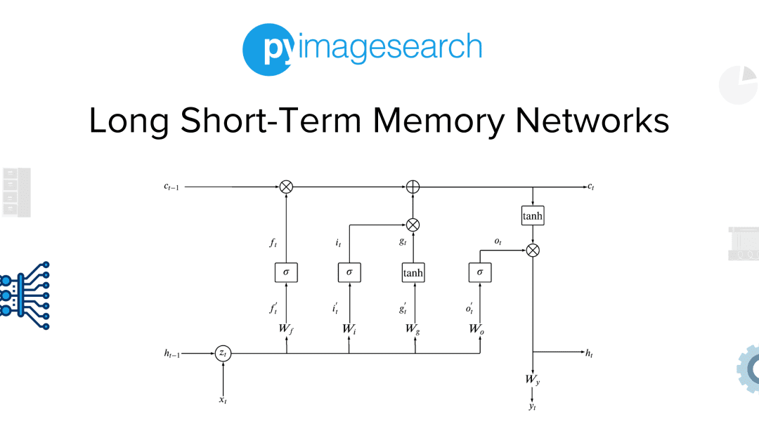
In this section, we see how to attain a better gradient flow with LSTMs. Let’s consider the following Figure 3 as the diagram of LSTM.

When we started with LSTMs, the image and formulae were not intuitive to us at all. If you feel lost here, we can assure you things will ease up as we go a little further.

The LSTM cell has two recurrence states, , the memory highway, and the , the hidden state representation. During feedforward, the inputs and are concatenated as a single vector for the simplicity and efficiency of calculations.

This input is then passed through multiple gates. The functions , , , are termed as gates of the LSTM architecture. They provide the intuition of how much a particular data needs to travel to represent it better.

A gate in the LSTM architecture is a multilayer perceptron with a non-linearity function. The choice of the non-linearity function will make sense as we study in-depth the different gates.

The Gates:

• Forget Gate : This gate is concerned with how much to forget. It takes in the input and then decides how much of the previous memory state should be forgotten. The activation non-linearity is . The gate’s output is 0 to 1. The 0 means to forget everything, while the 1 means to remember everything. This gate acts as a switch for the memory state circuit.
  
  
  
  After forgetting, we have the amount of memory state that we need from the previous step:
  
  

• Input gate : This gate decides how much of the present input needs to flow. This acts as a switch for the present input circuit. This gate also uses a non-linearity function.
  
  
  
• Gate gate : This gate closely resembles the recurrence formula of a vanilla RNN. We can say that this gate is the hidden state of the RNN in an LSTM. The resemblance to the RNN formula intensifies upon noticing the non-linearity function. This gate is the only one that uses a function.
  
  
  
  The Input gate and the Gate gate usage will make sense now. This is because the input gate behaves like a switch to the output of the Gate gate.
  
  
  
  Upon pointwise addition of and we get the present memory state. The memory state not only holds the past and present information but also holds a definite amount of both to make a better representation possible.
  
  

• Output gate : This gate is responsible for deciding how much output will flow into making the present hidden state.
  
  

• Let us pass the memory state from a first.
  
  

• Then the needs to be elementwise multiplied with the output gate to evaluate how much of the needs to be a part of the hidden state.
  
  

And now, we begin to build our LSTM model. But, first, let us go through the model.py file.

# import the necessary packages
from tensorflow.keras import layers
from tensorflow import keras

We begin with the necessary imports on Lines 1-3.

def get_lstm_model(vocabSize):
	# input for variable-length sequences of integers
	inputs = keras.Input(shape=(None,), dtype="int32")

	# embed the tokens in a 128-dimensional vector with masking
	# applied and apply dropout
	x = layers.Embedding(vocabSize, 128, mask_zero=True)(inputs)
	x = layers.Dropout(0.2)(x)

	# add 3 LSTMs
	x = layers.LSTM(64, return_sequences=True)(x)
	x = layers.LSTM(64, return_sequences=True)(x)
	x = layers.LSTM(64)(x)

	# add a classifier head
	x = layers.Dense(units=64, activation="relu")(x)
	x = layers.Dense(units=32, activation="relu")(x)
	x = layers.Dropout(0.2)(x)
	outputs = layers.Dense(1, activation="sigmoid")(x)
	
	# build the LSTM model
	model = keras.Model(inputs, outputs, name="LSTM")
	
	# return the LSTM model
	return model

On Line 31, we define the get_lstm_model that we use to create the model. Next, on Line 37, we pad and mask the variable length sequence and embed them on a 128-dimensional vector. For those who are a bit unclear about this, consider this 128-dimensional matrix as a way the computer views and assigns meaning to text.

On Line 38, we apply dropout to the inputs. Then, we add 3 simple LSTM cells on Lines 41-43 and a classifier head with a sigmoid activation on Lines 46-49.

Finally, the model is built using keras.Model API on Line 52 and returned on Line 55.

---

Vanishing and Exploding Gradients

Here, we see why LSTMs are preferred over RNNs.

Upon looking at Figure 4, we notice that the gradients of the memory state flow without much perturbation. Apart from the element-wise multiplication with the forget gate, the gradient flows freely in the circuit provided for the memory state.

LSTMs provide a gradient highway for the gradients to backpropagate efficiently. This makes the architecture robust to vanishing or exploding gradients.

---

Training and Visualizations

With the model created and ready, we can finally begin our training procedure. But before that, we must first look at some helper functions that will assist with visualizations and saving.

We begin with a function inside plot.py that will help us plot the loss and accuracy.

# import the necessary packages
import matplotlib.pyplot as plt

def plot_loss_accuracy(history, filepath):
	# plot the training and validation loss
	plt.style.use("ggplot")
	(fig, axs) = plt.subplots(2, 1)
	axs[0].plot(history["loss"], label="train_loss")
	axs[0].plot(history["val_loss"], label="val_loss")
	axs[0].set_xlabel("Epoch #")
	axs[0].set_ylabel("Loss")
	axs[0].legend()
	axs[1].plot(history["accuracy"], label="train_accuracy")
	axs[1].plot(history["val_accuracy"], label="val_accuracy")
	axs[1].set_xlabel("Epoch #")
	axs[1].set_ylabel("Accuracy")
	axs[1].legend()
	fig.savefig(filepath)

On Line 2, we begin by importing matplotlib. Then, on Line 4, we define the plot_loss_accuracy function that takes the model history and filepath as input.

Next, on Lines 6-17, we plot the loss and accuracy for training and validation and save the figure in the specified filepath on Line 18.

Next, we define another helper function called save_load.py to save the adapted vectorization layer for later use.

from tensorflow.keras.layers import TextVectorization
import tensorflow as tf
import pickle

def save_vectorizer(vectorizer, name):
	# pickle the weights of the vectorization layer
	pickle.dump({"weights": vectorizer.get_weights()},
		open(f"{name}.pkl", "wb"))

We begin with the necessary imports on Lines 1-3. Next, we define a function called save_vectorizer on Lines 5-8 that pickles and saves the weight of the vectorization layer.

And finally, with all the necessary functions defined, we can start with train.py, where we actually train our LSTM model.

# set the seed for reproducibility
import tensorflow as tf
tf.keras.utils.set_random_seed(42)

# import the necessary packages
from pyimagesearch.standardization import custom_standardization
from pyimagesearch.plot import plot_loss_accuracy
from pyimagesearch.save_load import save_vectorizer
from pyimagesearch.dataset import get_imdb_dataset
from pyimagesearch.model import get_rnn_model
from pyimagesearch.model import get_lstm_model
from pyimagesearch import config
from tensorflow.keras import layers
from tensorflow import keras
import os

We begin with all the necessary imports on Lines 5-18.

# get the IMDB dataset
print("[INFO] getting the IMDB dataset...")
(trainDs, valDs) = get_imdb_dataset(folderName=config.DATASET_PATH,
	batchSize=config.BATCH_SIZE, bufferSize=config.BUFFER_SIZE,
	autotune=tf.data.AUTOTUNE, test=False)

# initialize the text vectorization layer
vectorizeLayer = layers.TextVectorization(
	max_tokens=config.VOCAB_SIZE,
	output_mode="int",
	output_sequence_length=config.MAX_SEQUENCE_LENGTH,
	standardize=custom_standardization,
)

# grab the text from the training dataset and adapt the text
# vectorization layer on it
trainText = trainDs.map(lambda text, label: text)
vectorizeLayer.adapt(trainText)

# vectorize the training and the validation dataset
trainDs = trainDs.map(lambda text, label: (vectorizeLayer(text), label))
valDs = valDs.map(lambda text, label: (vectorizeLayer(text), label))

Next, on Lines 22-24, we get the IMDb dataset for movie reviews.

On Lines 27-32, we initialize the text vectorization layer with:

• max_tokens: The maximum number of tokens inside the vocabulary.
• output_mode: The data type for the output.
• output_sequence_length: The maximum sequence length needed for padding and masking.
• standardize: The custom standardization function that we defined previously.

On Lines 36 and 37, we adapt the vectorization layer on the training dataset.

When a text vectorization layer is initialized, it does not hold any information about the vocabulary of the training corpus. Therefore, to build a vocabulary, we need to pass the entire training dataset through the vectorization layer. This is known as adapting to the text.

Finally, on Lines 40-41, we vectorize the text of the training and validation dataset using the adapted vectorization layer.

# get the LSTM model and compile it
print("[INFO] building the LSTM model...")
modelLSTM = get_lstm_model(vocabSize=config.VOCAB_SIZE)
modelLSTM.compile(metrics=["accuracy"],
	optimizer=keras.optimizers.Adam(learning_rate=config.LR),
	loss=keras.losses.BinaryCrossentropy(from_logits=False),
)

# train the LSTM model
print("[INFO] training the LSTM model...")
historyLSTM = modelLSTM.fit(trainDs, epochs=config.EPOCHS,
	validation_data=valDs,
)

On Lines 59-63, we initialize the predefined LSTM model and compile it with Adam optimizer and Binary Cross Entropy loss.

On Lines 66-69, we fit the model on the training data and save its history onto the historyLSTM variable.

# check whether the output folder exists, if not build the output folder
if not os.path.exists(config.OUTPUT_PATH):
	os.makedirs(config.OUTPUT_PATH)

# save the loss and accuracy plots of RNN and LSTM models
plot_loss_accuracy(history=historyRNN.history, filepath=config.RNN_PLOT)
plot_loss_accuracy(history=historyLSTM.history, filepath=config.LSTM_PLOT)

On Line 72, we check whether the output path exists or create it otherwise. Finally, the plot_loss_accuracy function is called on Line 77 to visualize the loss and accuracy of the model.

# save the trained RNN and LSTM models to disk
print(f"[INFO] saving the RNN model to {config.RNN_MODEL_PATH}...")
keras.models.save_model(model=modelRNN, filepath=config.RNN_MODEL_PATH,
	include_optimizer=False)
print(f"[INFO] saving the LSTM model to {config.LSTM_MODEL_PATH}...")
keras.models.save_model(model=modelLSTM, filepath=config.LSTM_MODEL_PATH,
	include_optimizer=False)

On Lines 84 and 85, we then save the trained LSTM model on our disk.

# save the text vectorization layer to disk
save_vectorizer(vectorizer=vectorizeLayer, name=config.TEXT_VEC_PATH)

Finally, on Line 88, we save the text vectorization layer we used to vectorize the training and validation data.

We can verify the training and validation loss and accuracy from the model output. We have a 76% validation accuracy in just 10 epochs!

$ python train.py
[INFO] getting the IMDB dataset...
[INFO] building the LSTM model...
[INFO] training the LSTM model...
Epoch 1/10
22/22 [==============================] - 17s 280ms/step - loss: 0.6930 - accuracy: 0.5186 - val_loss: 0.6928 - val_accuracy: 0.5404
Epoch 2/10
22/22 [==============================] - 3s 116ms/step - loss: 0.6921 - accuracy: 0.5573 - val_loss: 0.6908 - val_accuracy: 0.5964
Epoch 3/10
22/22 [==============================] - 3s 121ms/step - loss: 0.6862 - accuracy: 0.6190 - val_loss: 0.6782 - val_accuracy: 0.6412
Epoch 4/10
22/22 [==============================] - 3s 123ms/step - loss: 0.6477 - accuracy: 0.6833 - val_loss: 0.6103 - val_accuracy: 0.6968
Epoch 5/10
22/22 [==============================] - 3s 119ms/step - loss: 0.5502 - accuracy: 0.7417 - val_loss: 0.5463 - val_accuracy: 0.7116
Epoch 6/10
22/22 [==============================] - 3s 123ms/step - loss: 0.4768 - accuracy: 0.7838 - val_loss: 0.5241 - val_accuracy: 0.7440
Epoch 7/10
22/22 [==============================] - 3s 117ms/step - loss: 0.4233 - accuracy: 0.8175 - val_loss: 0.5087 - val_accuracy: 0.7508
Epoch 8/10
22/22 [==============================] - 3s 118ms/step - loss: 0.3846 - accuracy: 0.8417 - val_loss: 0.5108 - val_accuracy: 0.7532
Epoch 9/10
22/22 [==============================] - 3s 119ms/step - loss: 0.3502 - accuracy: 0.8606 - val_loss: 0.5175 - val_accuracy: 0.7720
Epoch 10/10
22/22 [==============================] - 3s 121ms/step - loss: 0.3237 - accuracy: 0.8730 - val_loss: 0.5280 - val_accuracy: 0.7612
[INFO] saving the RNN model to output/rnn_model...
[INFO] saving the LSTM model to output/lstm_model...

---

Loading and Inference

Now that the model has been trained and saved to disk, we need to perform inference to understand the model performance. However, before starting with inference, let us first open save_load.py again and look at the load_vectorizer function.

def load_vectorizer(name, maxTokens, outputLength, standardize=None):
	# load the pickles data
	fromDisk = pickle.load(open(f"{name}.pkl", "rb"))

	# build a new vectorization layer
	newVectorizer = TextVectorization(max_tokens=maxTokens,
		output_mode="int", output_sequence_length=outputLength,
		standardize=standardize)

	# call the adapt method with some dummy data for the vectorization
	# layer to initialize properly
	newVectorizer.adapt(tf.data.Dataset.from_tensor_slices(["xyz"]))
	newVectorizer.set_weights(fromDisk["weights"])

	# return the vectorization layer
	return newVectorizer 

We define the load_vectorizer function on Line 10, which takes the following input:

• name: the filepath of the saved TextVectorization layer weights
• maxTokens: the maximum number of tokens in the vocabulary
• outputLength: the length of the output sequence
• standardize: we do not need any standardization function here

In the training pipeline, we build a TextVectorization layer to tokenize and vectorize our training data. In the inference pipeline, we need the same TextVectorization layer as the training pipeline.

We save the weights of the adapted TextVectorization layer and load the weights on top of a newly initialized layer. On Line 12, we load the weights of the saved TextVectorization layer. On Line 25, we return the loaded vectorizer.

# USAGE
# python inference.py

# import the necessary packages
from pyimagesearch.standardization import custom_standardization
from pyimagesearch.save_load import load_vectorizer
from pyimagesearch.dataset import get_imdb_dataset
from pyimagesearch import config
from tensorflow import keras
import tensorflow as tf

On Lines 1-10, we import the necessary packages.

print("[INFO] loading the pre-trained LSTM model...")
modelLstm = keras.models.load_model(filepath=config.LSTM_MODEL_PATH)
modelLstm.compile(optimizer="adam", metrics=["accuracy"],
	loss=keras.losses.BinaryCrossentropy(from_logits=False),
)

# get the IMDB dataset
print("[INFO] getting the IMDB test dataset...")
testDs = get_imdb_dataset(folderName=config.DATASET_PATH,
	batchSize=config.BATCH_SIZE, bufferSize=config.BUFFER_SIZE,
	autotune=tf.data.AUTOTUNE, test=True)

# load the pre-trained text vectorization layer
vectorizeLayer = load_vectorizer(name=config.TEXT_VEC_PATH,
	maxTokens=config.VOCAB_SIZE,
	outputLength=config.MAX_SEQUENCE_LENGTH,
	standardize=custom_standardization)

# vectorize the test dataset
testDs = testDs.map(lambda text, label: (vectorizeLayer(text), label))

# evaluate the trained RNN and LSTM model on the test dataset
for model in [modelRnn, modelLstm]:
	print(f"[INFO] test evaluation for {model.name}:")
	(testLoss, testAccuracy) = model.evaluate(testDs)
	print(f"\t[INFO] test loss: {testLoss:0.2f}")
	print(f"\t[INFO] test accuracy: {testAccuracy * 100:0.2f}%")

On Line 19, the saved LSTM model is loaded back to disk. The loaded model is then compiled with the suitable metrics, loss, and optimizer on Line 20.

On Lines 26-28, we get the testing dataset and pre-process it. Finally, Line 37 will map the dataset to get the vectorized tokens and labels.

On Lines 40-44, we evaluate the testing accuracy and loss of the LSTM model. Our model achieves 74.5% accuracy at inference!

$ python inference.py
[INFO] loading the pre-trained LSTM model...
[INFO] getting the IMDB test dataset...
[INFO] test evaluation for LSTM:
2022-04-04 13:04:26.163129: I tensorflow/stream_executor/cuda/cuda_dnn.cc:368] Loaded cuDNN version 8202
25/25 [==============================] - 8s 71ms/step - loss: 0.5660 - accuracy: 0.7450
        [INFO] test loss: 0.57
        [INFO] test accuracy: 74.50%

---

---

Summary

This brings us to the end of this tutorial on Long Short-Term Memory Networks. We started with RNNs and examined the reason why they failed. We also learned about an efficient solution in LSTMs. But this is not the end of the journey of sequence modeling. In fact, we are just getting started.

Imagine, for a moment, that you are not only able to predict which word comes where in the sentence but also how much that word contributes to the overall meaning of the sentence.

This sounds like a game changer, and it is. This concept is called attention, and we will discuss it in the next tutorial.

---

Citation Information

A. R. Gosthipaty, D. Chakraborty, and R. Raha. “Long Short-Term Memory Networks,” PyImageSearch, P. Chugh, S. Huot, K. Kidriavsteva, and A. Thanki, eds., 2022, https://pyimg.co/wtby9

@incollection{ADR_2022_LSTM,
  author = {Aritra Roy Gosthipaty and Devjyoti Chakraborty and Ritwik Raha},
  title = {Long Short-Term Memory Networks},
  booktitle = {PyImageSearch},
  editor = {Puneet Chugh and Susan Huot and Kseniia Kidriavsteva and Abhishek Thanki},
  year = {2022},
  note = {https://pyimg.co/wtby9},
}

---

To download the source code to this post (and be notified when future tutorials are published here on PyImageSearch), simply enter your email address in the form below!