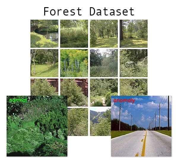
In this tutorial, you will learn how to perform anomaly/novelty detection in image datasets using OpenCV, Computer Vision, and the scikit-learn machine learning library.
Imagine this — you’re fresh out of college with a degree in Computer Science. You focused your studies specifically on computer vision and machine learning.
Your first job out of school is with the United States National Parks department.
Your task?
Build a computer vision system that can automatically recognize flower species in the park. Such a system can be used to detect invasive plant species that may be harmful to the overall ecosystem of the park.
You recognize immediately that computer vision can be used to recognize flower species.
But first you need to:
- Gather example images of each flower species in the park (i.e., build a dataset).
- Quantify the image dataset and train a machine learning model to recognize the species.
- Spot when outlier/anomaly plant species are detected, that way a trained botanist can inspect the plant and determine if it’s harmful to the park’s environment.
Steps #1 and #2 and fairly straightforward — but Step #3 is substantially harder to perform.
How are you supposed to train a machine learning model to automatically detect if a given input image is outside the “normal distribution” of what plants look like in the park?
The answer lies in a special class of machine learning algorithms, including outlier detection and novelty/anomaly detection.
In the remainder of this tutorial, you’ll learn the difference between these algorithms and how you can use them to spot outliers and anomalies in your own image datasets.
To learn how to perform anomaly/novelty detection in image datasets, just keep reading!
Intro to anomaly detection with OpenCV, Computer Vision, and scikit-learn
In the first part of this tutorial, we’ll discuss the difference between standard events that occur naturally and outlier/anomaly events.
We’ll also discuss why these types of events can be especially hard for machine learning algorithms to detect.
From there we’ll review our example dataset for this tutorial.
I’ll then show you how to:
- Load our input images from disk.
- Quantify them.
- Train a machine learning model used for anomaly detection on our quantified images.
- From there we’ll be able to detect outliers/anomalies in new input images.
Let’s get started!
What are outliers and anomalies? And why are they hard to detect?

Anomalies are defined as events that deviate from the standard, rarely happen, and don’t follow the rest of the “pattern”.
Examples of anomalies include:
- Large dips and spikes in the stock market due to world events
- Defective items in a factory/on a conveyor belt
- Contaminated samples in a lab
If you were to think of a bell curve, anomalies exist on the far, far ends of the tails.
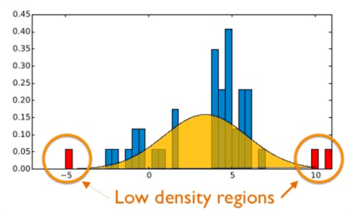
These events will occur, but will happen with an incredibly small probability.
From a machine learning perspective, this makes detecting anomalies hard — by definition, we have many examples of “standard” events and few examples of “anomaly” events.
We, therefore, have a massive skew in our dataset.
How are machine learning algorithms, which tend to work optimally with balanced datasets, supposed to work when the anomalies we want to detect may only happen 1%, 0.1%, or 0.0001% of the time?
Luckily, machine learning researchers have investigated this type of problem and have devised algorithms to handle the task.
Anomaly detection algorithms

Anomaly detection algorithms can be broken down into two subclasses:
- Outlier detection: Our input dataset contains examples of both standard events and anomaly events. These algorithms seek to fit regions of the training data where the standard events are most concentrated, disregarding, and therefore isolating, the anomaly events. Such algorithms are often trained in an unsupervised fashion (i.e., without labels). We sometimes use these methods to help clean and pre-process datasets before applying additional machine learning techniques.
- Novelty detection: Unlike outlier detection, which includes examples of both standard and anomaly events, novelty detection algorithms have only the standard event data points (i.e., no anomaly events) during training time. During training, we provide these algorithms with labeled examples of standard events (supervised learning). At testing/prediction time novelty detection algorithms must detect when an input data point is an outlier.
Outlier detection is a form of unsupervised learning. Here we provide our entire dataset of example data points and ask the algorithm to group them into inliers (standard data points) and outliers (anomalies).
Novelty detection is a form of supervised learning, but we only have labels for the standard data points — it’s up to the novelty detection algorithm to predict if a given data point is an inlier or outlier at test time.
In the remainder of this blog post, we’ll be focusing on novelty detection as a form of anomaly detection.
Isolation Forests for anomaly detection
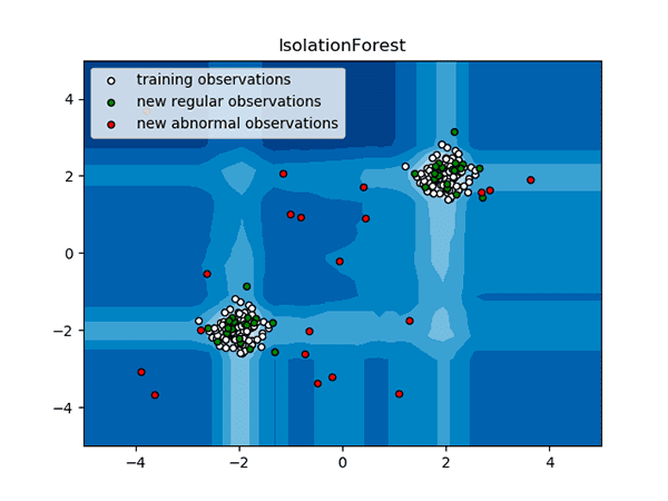
We’ll be using Isolation Forests to perform anomaly detection, based on Liu et al.’s 2012 paper, Isolation-Based Anomaly Detection.
Isolation forests are a type of ensemble algorithm and consist of multiple decision trees used to partition the input dataset into distinct groups of inliers.
As Figure 4 shows above, Isolation Forests accept an input dataset (white points) and then build a manifold surrounding them.
At test time, the Isolation Forest can then determine if the input points fall inside the manifold (standard events; green points) or outside the high-density area (anomaly events; red points).
Reviewing how the Isolation Forests constructs an ensemble of partitioning trees is outside the scope of this post, so be sure to refer to Liu et al.’s paper for more details.
Configuring your anomaly detection development environment
To follow along with today’s tutorial, you will need a Python 3 virtual environment with the following packages installed:
Luckily, each of these packages is pip-installable, but there are a handful of pre-requisites (including Python virtual environments). Be sure to follow the following guide first to set up your virtual environment with OpenCV: pip install opencv
Once your Python 3 virtual environment is ready, the pip install commands include:
$ workon <env-name>
$ pip install numpy
$ pip install opencv-contrib-python
$ pip install imutils
$ pip install scikit-learn
Note: The workon command becomes available once you install virtualenv and virtualenvwrapper per the pip install opencv installation guide.
Project structure
Be sure to grab the source code and example images to today’s post using the “Downloads” section of the tutorial. After you unarchive the .zip file you’ll be presented with the following project structure:
$ tree --dirsfirst
.
├── examples
│   ├── coast_osun52.jpg
│   ├── forest_cdmc290.jpg
│   └── highway_a836030.jpg
├── forest
│   ├── forest_bost100.jpg
│   ├── forest_bost101.jpg
│   ├── forest_bost102.jpg
│   ├── forest_bost103.jpg
│   ├── forest_bost98.jpg
│   ├── forest_cdmc458.jpg
│   ├── forest_for119.jpg
│   ├── forest_for121.jpg
│   ├── forest_for127.jpg
│   ├── forest_for130.jpg
│   ├── forest_for136.jpg
│   ├── forest_for137.jpg
│   ├── forest_for142.jpg
│   ├── forest_for143.jpg
│   ├── forest_for146.jpg
│   └── forest_for157.jpg
├── pyimagesearch
│   ├── __init__.py
│   └── features.py
├── anomaly_detector.model
├── test_anomaly_detector.py
└── train_anomaly_detector.py

3 directories, 24 files
Our project consists of forest/ images and example/ testing images. Our anomaly detector will try to determine if any of the three examples is an anomaly compared to the set of forest images.
Inside the pyimagesearch module is a file named features.py . This script contains two functions responsible for loading our image dataset from disk and calculating the color histogram features for each image.
We will operate our system in two stages — (1) training, and (2) testing.
First, the train_anomaly_detector.py script calculates features and trains an Isolation Forests machine learning model for anomaly detection, serializing the result as anomaly_detector.model .
Then we’ll develop test_anomaly_detector.py which accepts an example image and determines if it is an anomaly.
Our example image dataset
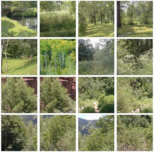
Our example dataset for this tutorial includes 16 images of forests (each of which is shown in Figure 5 above).
These example images are a subset of the 8 Scenes Dataset from Oliva and Torralba’s paper, Modeling the shape of the scene: a holistic representation of the spatial envelope.
We’ll take this dataset and train an anomaly detection algorithm on top of it.
When presented with a new input image, our anomaly detection algorithm will return one of two values:
1: “Yep, that’s a forest.”-1: “No, doesn’t look like a forest. It must be an outlier.”
You can thus think of this model as a “forest” vs “not forest” detector.
This model was trained on forest images and now must decide if a new input image fits inside the “forest manifold” or if is truly an anomaly/outlier.
To evaluate our anomaly detection algorithm we have 3 testing images:

As you can see, only one of these images is a forest — the other two are examples of highways and beach coasts, respectively.
If our anomaly detection pipeline is working properly, our model should return 1 (inlier) for the forest image and -1 for the two non-forest images.
Implementing our feature extraction and dataset loader helper functions
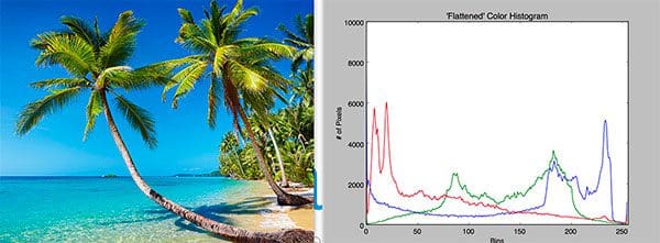
Before we can train a machine learning model to detect anomalies and outliers, we must first define a process to quantify and characterize the contents of our input images.
To accomplish this task, we’ll be using color histograms.
Color histograms are simple yet effective methods to characterize the color distribution of an image.
Since our task here is to characterize forest vs. non-forest images, we may assume that forest images will contain more shades of green versus their non-forest counterparts.
Let’s take a look at how we can implement color histogram extraction using OpenCV.
Open up the features.py file in the pyimagesearch module and insert the following code:
# import the necessary packages
from imutils import paths
import numpy as np
import cv2

def quantify_image(image, bins=(4, 6, 3)):
	# compute a 3D color histogram over the image and normalize it
	hist = cv2.calcHist([image], [0, 1, 2], None, bins,
		[0, 180, 0, 256, 0, 256])
	hist = cv2.normalize(hist, hist).flatten()

	# return the histogram
	return hist
Lines 2-4 import our packages. We’ll use paths from my imutils package to list all images in an input directory. OpenCV will be used to calculate and normalize histograms. NumPy is used for array operations.
Now that imports are taken care of, let’s define the quantify_image function. This function accepts two parameters:
image: The OpenCV-loaded image.bins: When plotting the histogram, the x-axis serves as our “bins.” In this case ourdefaultspecifies4hue bins,6saturation bins, and3value bins. Here’s a brief example — if we use only 2 (equally spaced) bins, then we are counting the number of times a pixel is in the range [0, 128] or [128, 255]. The number of pixels binned to the x-axis value is then plotted on the y-axis.
Note: To learn more about both histograms and color spaces including HSV, RGB, and L*a*b, and Grayscale, be sure to refer to Practical Python and OpenCV and PyImageSearch Gurus.
Lines 8-10 compute the color histogram and normalize it. Normalization allows us to count percentage and not raw frequency counts, helping in the case that some images are larger or smaller than others.
Line 13 returns the normalized histogram to the caller.
Our next function handles:
- Accepting the path to a directory containing our dataset of images.
- Looping over the image paths while quantifying them using our
quantify_imagemethod.
Let’s take a look at this method now:
def load_dataset(datasetPath, bins):
	# grab the paths to all images in our dataset directory, then
	# initialize our lists of images
	imagePaths = list(paths.list_images(datasetPath))
	data = []

	# loop over the image paths
	for imagePath in imagePaths:
		# load the image and convert it to the HSV color space
		image = cv2.imread(imagePath)
		image = cv2.cvtColor(image, cv2.COLOR_BGR2HSV)

		# quantify the image and update the data list
		features = quantify_image(image, bins)
		data.append(features)

	# return our data list as a NumPy array
	return np.array(data)
Our load_dataset function accepts two parameters:
datasetPath: The path to our dataset of images.bins: Num of bins for the color histogram. Refer to the explanation above. The bins are passed to thequantify_imagefunction.
Line 18 grabs all image paths in the datasetPath .
Line 19 initializes a list to hold our features data .
From there, Line 22 begins a loop over the imagePaths . Inside the loop we load an image and convert it to the HSV color space (Lines 24 and 25). Then we quantify the image , and add the resulting features to the data list (Lines 28 and 29).
Finally, Line 32 returns our data list as a NumPy array to the caller.
Implementing our anomaly detection training script with scikit-learn
With our helper functions implemented we can now move on to training an anomaly detection model.
As mentioned earlier in this tutorial, we’ll be using an Isolation Forest to help determine anomaly/novelty data points.
Our implementation of Isolation Forests comes from the scikit-learn library.
Open up the train_anomaly_detector.py file and let’s get to work:
# import the necessary packages
from pyimagesearch.features import load_dataset
from sklearn.ensemble import IsolationForest
import argparse
import pickle

# construct the argument parser and parse the arguments
ap = argparse.ArgumentParser()
ap.add_argument("-d", "--dataset", required=True,
	help="path to dataset of images")
ap.add_argument("-m", "--model", required=True,
	help="path to output anomaly detection model")
args = vars(ap.parse_args())
Lines 2-6 handle our imports. This script uses our custom load_dataset function and scikit-learn’s implementation of Isolation Forests. We’ll serialize our resulting model as a pickle file.
Lines 8-13 parse our command line arguments including:
--dataset: The path to our dataset of images.--model: The path to the output anomaly detection model.
At this point, we’re ready to load our dataset and train our Isolation Forest model:
# load and quantify our image dataset
print("[INFO] preparing dataset...")
data = load_dataset(args["dataset"], bins=(3, 3, 3))

# train the anomaly detection model
print("[INFO] fitting anomaly detection model...")
model = IsolationForest(n_estimators=100, contamination=0.01,
	random_state=42)
model.fit(data)
Line 17 loads and quantifies the image dataset.
Lines 21 and 22 initializes our IsolationForest model with the following parameters:
n_estimators: The number of base estimators (i.e., trees) in the ensemble.contamination: The proportion of outliers in the dataset.random_state: The random number generator seed value for reproducibility. You can use any integer;42is commonly used in the machine learning world as it relates to a joke in the book, Hitchhiker’s Guide to the Galaxy.
Be sure to refer to other optional parameters to the Isolation Forest in the scikit-learn documentation.
Line 23 trains the anomaly detector on top of the histogram data .
Now that our model is trained, the remaining lines serialize the anomaly detector to a pickle file on disk:
# serialize the anomaly detection model to disk
f = open(args["model"], "wb")
f.write(pickle.dumps(model))
f.close()
Training our anomaly detector
Now that we have implemented our anomaly detection training script, let’s put it to work.
Start by making sure you have used the “Downloads” section of this tutorial to download the source code and example images.
From there, open up a terminal and execute the following command:
$ python train_anomaly_detector.py --dataset forest --model anomaly_detector.model
[INFO] preparing dataset...
[INFO] fitting anomaly detection model...
To verify that the anomaly detector has been serialized to disk, check the contents of your working project directory:
$ ls *.model
anomaly_detector.model
Creating the anomaly detector testing script
At this point we have trained our anomaly detection model — but how do we use to actually detect anomalies in new data points?
To answer that question, let’s look at the test_anomaly_detector.py script.
At a high-level, this script:
- Loads the anomaly detection model trained in the previous step.
- Loads, preprocesses, and quantifies a query image.
- Makes a prediction with our anomaly detector to determine if the query image is an inlier or an outlier (i.e. anomaly).
- Displays the result.
Go ahead and open test_anomaly_detector.py and insert the following code:
# import the necessary packages
from pyimagesearch.features import quantify_image
import argparse
import pickle
import cv2

# construct the argument parser and parse the arguments
ap = argparse.ArgumentParser()
ap.add_argument("-m", "--model", required=True,
	help="path to trained anomaly detection model")
ap.add_argument("-i", "--image", required=True,
	help="path to input image")
args = vars(ap.parse_args())
Lines 2-5 handle our imports. Notice that we import our custom quantify_image function to calculate features on our input image. We also import pickle to load our anomaly detection model. OpenCV will be used for loading, preprocessing, and displaying images.
Our script requires two command line arguments:
--model: The serialized anomaly detector residing on disk.--image: The path to the input image (i.e. our query).
Let’s load our anomaly detector and quantify our input image:
# load the anomaly detection model
print("[INFO] loading anomaly detection model...")
model = pickle.loads(open(args["model"], "rb").read())

# load the input image, convert it to the HSV color space, and
# quantify the image in the *same manner* as we did during training
image = cv2.imread(args["image"])
hsv = cv2.cvtColor(image, cv2.COLOR_BGR2HSV)
features = quantify_image(hsv, bins=(3, 3, 3))
Line 17 loads our pre-trained anomaly detector.
Lines 21-23 load, preprocess, and quantify our input image . Our preprocessing steps must be the same as in our training script (i.e. converting from BGR to HSV color space).
At this point, we’re ready to make an anomaly prediction and display results:
# use the anomaly detector model and extracted features to determine
# if the example image is an anomaly or not
preds = model.predict([features])[0]
label = "anomaly" if preds == -1 else "normal"
color = (0, 0, 255) if preds == -1 else (0, 255, 0)

# draw the predicted label text on the original image
cv2.putText(image, label, (10,  25), cv2.FONT_HERSHEY_SIMPLEX,
	0.7, color, 2)

# display the image
cv2.imshow("Output", image)
cv2.waitKey(0)
Line 27 makes predictions on the input image features . Our anomaly detection model will return 1 for a “normal” data point and -1 for an “outlier”.
Line 28 assigns either an "anomaly" or "normal" label to our prediction.
Lines 32-37 then annotate the label onto the query image and display it on screen until any key is pressed.
Detecting anomalies in image datasets using computer vision and scikit-learn
To see our anomaly detection model in action make sure you have used the “Downloads” section of this tutorial to download the source code, example image dataset, and pre-trained model.
From there, you can use the following command to test the anomaly detector:
$ python test_anomaly_detector.py --model anomaly_detector.model \
	--image examples/forest_cdmc290.jpg
[INFO] loading anomaly detection model...
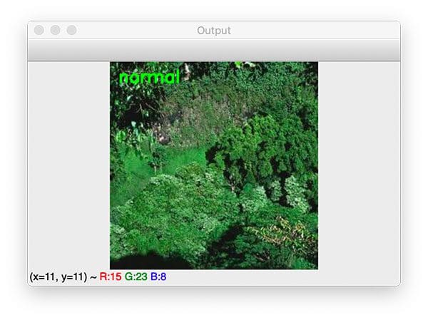
Here you can see that our anomaly detector has correctly labeled the forest as an inlier.
Let’s now see how the model handles an image of a highway, which is certainly not a forest:
$ python test_anomaly_detector.py --model anomaly_detector.model \
	--image examples/highway_a836030.jpg
[INFO] loading anomaly detection model...

Our anomaly detector correctly labels this image as an outlier/anomaly.
As a final test, let’s supply an image of a beach/coast to the anomaly detector:
$ python test_anomaly_detector.py --model anomaly_detector.model \
	--image examples/coast_osun52.jpg
[INFO] loading anomaly detection model...
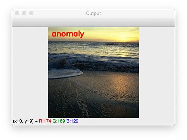
Once again, our anomaly detector correctly identifies the image as an outlier/anomaly.
What's next? We recommend PyImageSearch University.
86+ total classes • 115+ hours hours of on-demand code walkthrough videos • Last updated: June 2025
★★★★★ 4.84 (128 Ratings) • 16,000+ Students Enrolled
I strongly believe that if you had the right teacher you could master computer vision and deep learning.
Do you think learning computer vision and deep learning has to be time-consuming, overwhelming, and complicated? Or has to involve complex mathematics and equations? Or requires a degree in computer science?
That’s not the case.
All you need to master computer vision and deep learning is for someone to explain things to you in simple, intuitive terms. And that’s exactly what I do. My mission is to change education and how complex Artificial Intelligence topics are taught.
If you're serious about learning computer vision, your next stop should be PyImageSearch University, the most comprehensive computer vision, deep learning, and OpenCV course online today. Here you’ll learn how to successfully and confidently apply computer vision to your work, research, and projects. Join me in computer vision mastery.
Inside PyImageSearch University you'll find:
- ✓ 86+ courses on essential computer vision, deep learning, and OpenCV topics
- ✓ 86 Certificates of Completion
- ✓ 115+ hours hours of on-demand video
- ✓ Brand new courses released regularly, ensuring you can keep up with state-of-the-art techniques
- ✓ Pre-configured Jupyter Notebooks in Google Colab
- ✓ Run all code examples in your web browser — works on Windows, macOS, and Linux (no dev environment configuration required!)
- ✓ Access to centralized code repos for all 540+ tutorials on PyImageSearch
- ✓ Easy one-click downloads for code, datasets, pre-trained models, etc.
- ✓ Access on mobile, laptop, desktop, etc.
Summary
In this tutorial you learned how to perform anomaly and outlier detection in image datasets using computer vision and the scikit-learn machine learning library.
To perform anomaly detection, we:
- Gathered an example image dataset of forest images.
- Quantified the image dataset using color histograms and the OpenCV library.
- Trained an Isolation Forest on our quantified images.
- Used the Isolation Forest to detect image outliers and anomalies.
Along with Isolation Forests you should also investigate One-class SVMs, Elliptic Envelopes, and Local Outlier Factor algorithms as they can be used for outlier/anomaly detection as well.
But what about deep learning?
Can deep learning be used to perform anomaly detection too?
I’ll answer that question in a future tutorial.
To download the source code to this post (and be notified when future tutorials are published here on PyImageSearch), just enter your email address in the form below!

Download the Source Code and FREE 17-page Resource Guide
Enter your email address below to get a .zip of the code and a FREE 17-page Resource Guide on Computer Vision, OpenCV, and Deep Learning. Inside you'll find my hand-picked tutorials, books, courses, and libraries to help you master CV and DL!
