Convolution and cross-correlation in neural networks

Our entire review of machine learning and neural networks thus far has been leading up to this point: understanding Convolutional Neural Networks (CNNs) and the role they play in deep learning.

In traditional feedforward neural networks, each neuron in the input layer is connected to every output neuron in the next layer — we call this a fully connected (FC) layer. However, in CNNs, we don’t use FC layers until the very last layer(s) in the network. We can thus define a CNN as a neural network that swaps in a specialized “convolutional” layer in place of “fully connected” layer for at least one of the layers in the network (Goodfellow, Bengio, and Courville, 2016).

A nonlinear activation function, such as ReLU, is then applied to the output of these convolutions and the process of convolution => activation continues (along with a mixture of other layer types to help reduce the width and height of the input volume and help reduce overfitting) until we finally reach the end of the network and apply one or two FC layers where we can obtain our final output classifications.

Each layer in a CNN applies a different set of filters, typically hundreds or thousands of them, and combines the results, feeding the output into the next layer in the network. During training, a CNN automatically learns the values for these filters.

In the context of image classification, our CNN may learn to:

• Detect edges from raw pixel data in the first layer.
• Use these edges to detect shapes (i.e., “blobs”) in the second layer.
• Use these shapes to detect higher-level features such as facial structures, parts of a car, etc. in the highest layers of the network.

The last layer in a CNN uses these higher-level features to make predictions regarding the contents of the image. In practice, CNNs give us two key benefits: local invariance and compositionality. The concept of local invariance allows us to classify an image as containing a particular object regardless of where in the image the object appears. We obtain this local invariance through the usage of “pooling layers,” which identifies regions of our input volume with a high response to a particular filter.

The second benefit is compositionality. Each filter composes a local patch of lower-level features into a higher-level representation, similar to how we can compose a set of mathematical functions that build on the output of previous functions: f(g(h(x))) — this composition allows our network to learn more rich features deeper in the network. For example, our network may build edges from pixels, shapes from edges, and then complex objects from shapes — all in an automated fashion that happens naturally during the training process. The concept of building higher-level features from lower-level ones is exactly why CNNs are so powerful in computer vision.

Understanding Convolutions

In this section, we’ll address a number of questions, including:

• What are image convolutions?
• What do they do?
• Why do we use them?
• How do we apply them to images?
• And what role do convolutions play in deep learning?

The word “convolution” sounds like a fancy, complicated term — but it’s really not. If you have any prior experience with computer vision, image processing, or OpenCV before, you’ve already applied convolutions, whether you realize it or not!

Ever apply blurring or smoothing to an image? Yep, that’s a convolution. What about edge detection? Yup, convolution. Have you opened Photoshop or GIMP to sharpen an image? You guessed it — convolution. Convolutions are one of the most critical, fundamental building blocks in computer vision and image processing.

But the term itself tends to scare people off — in fact, on the surface, the word even appears to have a negative connotation (why would anyone want to “convolute” something?) Trust me, convolutions are anything but scary. They’re actually quite easy to understand.

In terms of deep learning, an (image) convolution is an element-wise multiplication of two matrices followed by a sum.

Seriously. That’s it. You just learned what a convolution is:

1. Take two matrices (which both have the same dimensions).
2. Multiply them, element-by-element (i.e., not the dot product, just a simple multiplication).
3. Sum the elements together.

Convolutions versus Cross-correlation

A reader with prior background in computer vision and image processing may have identified my description of a convolution above as a cross-correlation operation instead. Using cross-correlation instead of convolution is actually by design. Convolution (denoted by the operator) over a two-dimensional input image I and two-dimensional kernel K is defined as:

(1)

However, nearly all machine learning and deep learning libraries use the simplified cross-correlation function

(2)

All this math amounts to is a sign change in how we access the coordinates of the image I (i.e., we don’t have to “flip” the kernel relative to the input when applying cross-correlation).

Again, many deep learning libraries use the simplified cross-correlation operation and call it convolution — we will use the same terminology here. For readers interested in learning more about the mathematics behind convolution vs. cross-correlation, please refer to Chapter 3 of Computer Vision: Algorithms and Applications by Szeliski (2011).

The “Big Matrix” and “Tiny Matrix” Analogy

An image is a multidimensional matrix. Our image has a width (# of columns) and height (# of rows), just like a matrix. But unlike traditional matrices you have worked with back in grade school, images also have a depth to them — the number of channels in the image.

For a standard RGB image, we have a depth of 3 — one channel for each of the Red, Green, and Blue channels, respectively. Given this knowledge, we can think of an image as big matrix and a kernel or convolutional matrix as a tiny matrix that is used for blurring, sharpening, edge detection, and other processing functions. Essentially, this tiny kernel sits on top of the big image and slides from left-to-right and top-to-bottom, applying a mathematical operation (i.e., a convolution) at each (x, y)-coordinate of the original image.

It’s normal to hand-define kernels to obtain various image processing functions. In fact, you might already be familiar with blurring (average smoothing, Gaussian smoothing, etc.), edge detection (Laplacian, Sobel, Scharr, Prewitt, etc.), and sharpening — all of these operations are forms of hand-defined kernels that are specifically designed to perform a particular function.

So that raises the question: is there a way to automatically learn these types of filters? And even use these filters for image classification and object detection? You bet there is. But before we get there, we need to understand kernels and convolutions a bit more.

Kernels

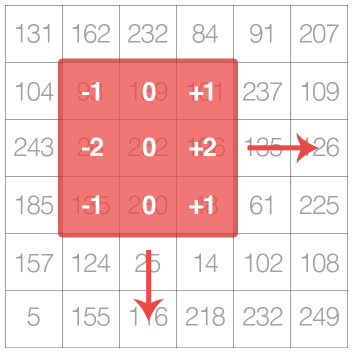
Again, let’s think of an image as a big matrix and a kernel as a tiny matrix (at least in respect to the original “big matrix” image), depicted in Figure 1. As the figure demonstrates, we are sliding the kernel (red region) from left-to-right and top-to-bottom along the original image. At each (x, y)-coordinate of the original image, we stop and examine the neighborhood of pixels located at the center of the image kernel. We then take this neighborhood of pixels, convolve them with the kernel, and obtain a single output value. The output value is stored in the output image at the same (x, y)-coordinates as the center of the kernel.

Before we dive into an example, let’s take a look at what a kernel looks like (Equation (3)):

(3)

Above, we have defined a square 3×3 kernel (any guesses on what this kernel is used for?). Kernels can be of arbitrary rectangular size M×N, provided that both M and N are odd integers.

Remark: Most kernels applied to deep learning and CNNs are N×N square matrices, allowing us to take advantage of optimized linear algebra libraries that operate most efficiently on square matrices.

We use an odd kernel size to ensure there is a valid integer (x, y)-coordinate at the center of the image (Figure 2). On the left, we have a 3×3 matrix. The center of the matrix is located at x = 1, y = 1, where the top-left corner of the matrix is used as the origin and our coordinates are zero-indexed. But on the right, we have a 2×2 matrix. The center of this matrix would be located at x = 0.5, y = 0.5.

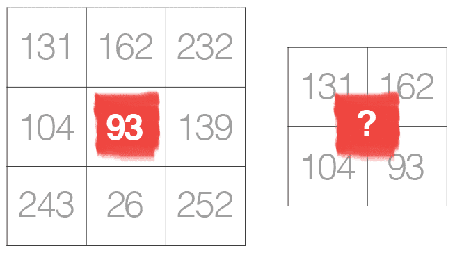
But as we know, without applying interpolation, there is no such thing as pixel location (0.5, 0.5) — our pixel coordinates must be integers! This reasoning is exactly why we use odd kernel sizes: to always ensure there is a valid (x, y)-coordinate at the center of the kernel.

A Hand Computation Example of Convolution

Now that we have discussed the basics of kernels, let’s discuss the actual convolution operation and see an example of it actually being applied to help us solidify our knowledge. In image processing, a convolution requires three components:

1. An input image.
2. A kernel matrix that we are going to apply to the input image.
3. An output image to store the output of the image convolved with the kernel.

Convolution (or cross-correlation) is actually very easy. All we need to do is:

1. Select an (x, y)-coordinate from the original image.
2. Place the center of the kernel at this (x, y)-coordinate.
3. Take the element-wise multiplication of the input image region and the kernel, then sum up the values of these multiplication operations into a single value. The sum of these multiplications is called the kernel output.
4. Use the same (x, y)-coordinates from Step #1, but this time, store the kernel output at the same (x, y)-location as the output image.

Below, you can find an example of convolving (denoted mathematically as the operator) a 3×3 region of an image with a 3×3 kernel used for blurring:

(4)

Therefore,

(5)

After applying this convolution, we would set the pixel located at the coordinate (i, j) of the output image O to O_{i, j} = 132.

That’s all there is to it! Convolution is simply the sum of element-wise matrix multiplication between the kernel and neighborhood that the kernel covers of the input image.

Implementing Convolutions with Python

To help us further understand the concept of convolutions, let’s look at some actual code that will reveal how kernels and convolutions are implemented. This source code will not only help you understand how to apply convolutions to images, but also enable you to understand what’s going on under the hood when training CNNs.

Open a new file, name it convolutions.py, and let’s get to work:

# import the necessary packages
from skimage.exposure import rescale_intensity
import numpy as np
import argparse
import cv2

We start on Lines 2-5 by importing our required Python packages. We will use NumPy and OpenCV for our standard numerical array processing and computer vision functions, along with the scikit-image library to help us implement our own custom convolution function.

Next, we can start defining this convolve method:

def convolve(image, K):
	# grab the spatial dimensions of the image and kernel
	(iH, iW) = image.shape[:2]
	(kH, kW) = K.shape[:2]

	# allocate memory for the output image, taking care to "pad"
	# the borders of the input image so the spatial size (i.e.,
	# width and height) are not reduced
	pad = (kW - 1) // 2
	image = cv2.copyMakeBorder(image, pad, pad, pad, pad,
		cv2.BORDER_REPLICATE)
	output = np.zeros((iH, iW), dtype="float")

The convolve function requires two parameters: the (grayscale) image that we want to convolve with kernel. Given both our image and kernel (which we presume to be NumPy arrays), we then determine the spatial dimensions (i.e., width and height) of each (Lines 9 and 10).

Before we continue, it’s important to understand the process of “sliding” a convolutional matrix across an image, applying the convolution, and then storing the output, which will actually decrease the spatial dimensions of our input image. Why is this?

Recall that we “center” our computation around the center (x, y)-coordinate of the input image that the kernel is currently positioned over. This positioning implies there is no such thing as “center” pixels for pixels that fall along the border of the image (as the corners of the kernel would be “hanging off” the image where the values are undefined), depicted by Figure 3.

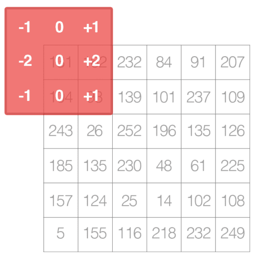
The decrease in spatial dimension is simply a side effect of applying convolutions to images. Sometimes this effect is desirable, and other times it is not, it simply depends on your application.

However, in most cases, we want our output image to have the same dimensions as our input image. To ensure the dimensions are the same, we apply padding (Lines 15-18). Here we are simply replicating the pixels along the border of the image, such that the output image will match the dimensions of the input image.

Other padding methods exist, including zero padding (filling the borders with zeros — very common when building Convolutional Neural Networks) and wrap around (where the border pixels are determined by examining the opposite side of the image). In most cases, you will see either replicate or zero padding. Replicate padding is more commonly used when aesthetics are concerned while zero padding is best for efficiency.

We are now ready to apply the actual convolution to our image:

	# loop over the input image, "sliding" the kernel across
	# each (x, y)-coordinate from left-to-right and top-to-bottom
	for y in np.arange(pad, iH + pad):
		for x in np.arange(pad, iW + pad):
			# extract the ROI of the image by extracting the
			# *center* region of the current (x, y)-coordinates
			# dimensions
			roi = image[y - pad:y + pad + 1, x - pad:x + pad + 1]

			# perform the actual convolution by taking the
			# element-wise multiplication between the ROI and
			# the kernel, then summing the matrix
			k = (roi * K).sum()

			# store the convolved value in the output (x, y)-
			# coordinate of the output image
			output[y - pad, x - pad] = k

Lines 22 and 23 loop over our image, “sliding” the kernel from left-to-right and top-to-bottom, one pixel at a time. Line 27 extracts the Region of Interest (ROI) from the image using NumPy array slicing. The roi will be centered around the current (x, y)-coordinates of the image. The roi will also have the same size as our kernel, which is critical for the next step.

Convolution is performed on Line 32 by taking the element-wise multiplication between the roi and kernel, followed by summing the entries in the matrix. The output value k is then stored in the output array at the same (x, y)-coordinates (relative to the input image).

We can now finish up our convolve method:

	# rescale the output image to be in the range [0, 255]
	output = rescale_intensity(output, in_range=(0, 255))
	output = (output * 255).astype("uint8")

	# return the output image
	return output

When working with images, we typically deal with pixel values falling in the range [0, 255]. However, when applying convolutions, we can easily obtain values that fall outside this range. In order to bring our output image back into the range [0, 255], we apply the rescale_intensity function of scikit-image (Line 39).

We also convert our image back to an unsigned 8-bit integer data type on Line 40 (previously, the output image was a floating point type in order to handle pixel values outside the range [0, 255]). Finally, the output image is returned to the calling function on Line 43.

Now that we’ve defined our convolve function, let’s move on to the driver portion of the script. This section of our lesson will handle parsing command line arguments, defining a series of kernels we are going to apply to our image, and then displaying the output results:

# construct the argument parse and parse the arguments
ap = argparse.ArgumentParser()
ap.add_argument("-i", "--image", required=True,
	help="path to the input image")
args = vars(ap.parse_args())

Our script requires only a single command line argument, --image, which is the path to our input image. We can then define two kernels used for blurring and smoothing an image:

# construct average blurring kernels used to smooth an image
smallBlur = np.ones((7, 7), dtype="float") * (1.0 / (7 * 7))
largeBlur = np.ones((21, 21), dtype="float") * (1.0 / (21 * 21))

To convince yourself that this kernel is performing blurring, notice how each entry in the kernel is an average of 1/S, where S is the total number of entries in the matrix. Thus, this kernel will multiply each input pixel by a small fraction and take the sum — this is exactly the definition of the average.

We then have a kernel responsible for sharpening an image:

# construct a sharpening filter
sharpen = np.array((
	[0, -1, 0],
	[-1, 5, -1],
	[0, -1, 0]), dtype="int")

Then the Laplacian kernel used to detect edge-like regions:

# construct the Laplacian kernel used to detect edge-like
# regions of an image
laplacian = np.array((
	[0, 1, 0],
	[1, -4, 1],
	[0, 1, 0]), dtype="int")

The Sobel kernels can be used to detect edge-like regions along both the x and y axis, respectively:

# construct the Sobel x-axis kernel
sobelX = np.array((
	[-1, 0, 1],
	[-2, 0, 2],
	[-1, 0, 1]), dtype="int")

# construct the Sobel y-axis kernel
sobelY = np.array((
	[-1, -2, -1],
	[0, 0, 0],
	[1, 2, 1]), dtype="int")

And finally, we define the emboss kernel:

# construct an emboss kernel
emboss = np.array((
	[-2, -1, 0],
	[-1, 1, 1],
	[0, 1, 2]), dtype="int")

Explaining how each of these kernels was formulated is outside the scope of this tutorial, so for the time being simply understand that these are kernels that were manually built to perform a given operation.

For a thorough treatment of how kernels are mathematically constructed and proven to perform a given image processing operation, please refer to Szeliski (Chapter 3). I also recommend using this excellent kernel visualization tool from Setosa.io.

Given all these kernels, we can lump them together into a set of tuples called a “kernel bank”:

# construct the kernel bank, a list of kernels we're going to apply
# using both our custom 'convolve' function and OpenCV's 'filter2D'
# function
kernelBank = (
	("small_blur", smallBlur),
	("large_blur", largeBlur),
	("sharpen", sharpen),
	("laplacian", laplacian),
	("sobel_x", sobelX),
	("sobel_y", sobelY),
	("emboss", emboss))

Constructing this list of kernels enables us to loop over them and visualize their output in an efficient manner, as the code block below demonstrates:

# load the input image and convert it to grayscale
image = cv2.imread(args["image"])
gray = cv2.cvtColor(image, cv2.COLOR_BGR2GRAY)

# loop over the kernels
for (kernelName, K) in kernelBank:
	# apply the kernel to the grayscale image using both our custom
	# 'convolve' function and OpenCV's 'filter2D' function
	print("[INFO] applying {} kernel".format(kernelName))
	convolveOutput = convolve(gray, K)
	opencvOutput = cv2.filter2D(gray, -1, K)

	# show the output images
	cv2.imshow("Original", gray)
	cv2.imshow("{} - convolve".format(kernelName), convolveOutput)
	cv2.imshow("{} - opencv".format(kernelName), opencvOutput)
	cv2.waitKey(0)
	cv2.destroyAllWindows()

Lines 99 and 100 load our image from disk and convert it to grayscale. Convolution operators can and are applied to RGB or other multi-channel volumes, but for the sake of simplicity, we’ll only apply our filters to grayscale images.

We start looping over our set of kernels in the kernelBank on Line 103 and then apply the current kernel to the gray image on Line 107 by calling our function convolve method, defined earlier in the script.

As a sanity check, we also call cv2.filter2D, which also applies our kernel to the gray image. The cv2.filter2D function is OpenCV’s much more optimized version of our convolve function. The main reason I am including both here is for us to sanity check our custom implementation.

Finally, Lines 111-115 display the output images on our screen for each kernel type.

Convolution Results

To run our script (and visualize the output of various convolution operations), just issue the following command:

$ python convolutions.py --image jemma.png

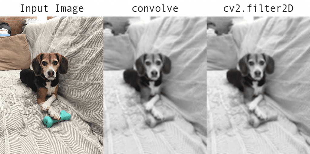
You’ll then see the results of applying the smallBlur kernel to the input image in Figure 4. On the left, we have our original image. Then, in the center, we have the results from the convolve function. And on the right, the results from cv2.filter2D. A quick visual inspection will reveal that our output matches cv2.filter2D, indicating that our convolve function is working properly. Furthermore, our image now appears “blurred” and “smoothed,” thanks to the smoothing kernel.

Let’s apply a larger blur, results of which can be seen in Figure 5 (top-left). This time I am omitting the cv2.filter2D results to save space. Comparing the results from Figure 5 to Figure 4, notice how as the size of the averaging kernel increases, the amount of blurring in the output image increases as well.

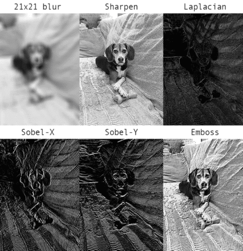
We can also sharpen our image (Figure 5, top-mid) and detect edge-like regions via the Laplacian operator (top-right).

The sobelX kernel is used to find vertical edges in the image (Figure 5, bottom-left), while the sobelY kernel reveals horizontal edges (bottom-mid). Finally, we can see the result of the emboss kernel in the bottom-right.

The Role of Convolutions in Deep Learning

We must manually hand-define each of our kernels for each of our various image processing operations, such as smoothing, sharpening, and edge detection. That’s all fine and good, but what if there was a way to learn these filters instead?

Is it possible to define a machine learning algorithm that can look at our input images and eventually learn these types of operators? In fact, there is — these types of algorithms are: Convolutional Neural Networks (CNNs).

By applying convolutional filters, nonlinear activation functions, pooling, and backpropagation, CNNs are able to learn filters that can detect edges and blob-like structures in lower-level layers of the network — and then use the edges and structures as “building blocks,” eventually detecting high-level objects (e.g., faces, cats, dogs, cups, etc.) in the deeper layers of the network.

This process of using the lower-level layers to learn high-level features is exactly the compositionality of CNNs that we were referring to earlier. But exactly how do CNNs do this? The answer is by stacking a specific set of layers in a purposeful manner. We will discuss these types of layers in a separate lesson, followed by examining common layer stacking patterns that are widely used among many image classification tasks.