Convolutional Neural Networks (CNNs) and Layer Types

CNN Building Blocks

Neural networks accept an input image/feature vector (one input node for each entry) and transform it through a series of hidden layers, commonly using nonlinear activation functions. Each hidden layer is also made up of a set of neurons, where each neuron is fully connected to all neurons in the previous layer. The last layer of a neural network (i.e., the “output layer”) is also fully connected and represents the final output classifications of the network.

A diverse dataset is essential for training a CNN and understanding its different layer types. By training the network on the dataset, we can observe how each layer extracts features and contributes to the final prediction.

Roboflow has free tools for each stage of the computer vision pipeline that will streamline your workflows and supercharge your productivity.

Sign up or Log in to your Roboflow account to access state of the art dataset libaries and revolutionize your computer vision pipeline.

You can start by choosing your own datasets or using our PyimageSearch’s assorted library of useful datasets.

Bring data in any of 40+ formats to Roboflow, train using any state-of-the-art model architectures, deploy across multiple platforms (API, NVIDIA, browser, iOS, etc), and connect to applications or 3rd party tools.

However, neural networks operating directly on raw pixel intensities:

1. Do not scale well as the image size increases.
2. Leaves much accuracy to be desired (i.e., a standard feedforward neural network on CIFAR-10 obtained only 52% accuracy).

To demonstrate how standard neural networks do not scale well as image size increases, let’s again consider the CIFAR-10 dataset. Each image in CIFAR-10 is 32×32 with a Red, Green, and Blue channel, yielding a total of 32×32×3 = 3,072 total inputs to our network.

A total of 3,072 inputs does not seem to amount to much, but consider if we were using 250×250 pixel images — the total number of inputs and weights would jump to 250×250×3 = 187,500 — and this number is only for the input layer alone! Surely, we would want to add multiple hidden layers with a varying number of nodes per layer — these parameters can quickly add up, and given the poor performance of standard neural networks on raw pixel intensities, this bloat is hardly worth it.

Instead, we can use Convolutional Neural Networks (CNNs) that take advantage of the input image structure and define a network architecture in a more sensible way. Unlike a standard neural network, layers of a CNN are arranged in a 3D volume in three dimensions: width, height, and depth (where depth refers to the third dimension of the volume, such as the number of channels in an image or the number of filters in a layer).

To make this example more concrete, again consider the CIFAR-10 dataset: the input volume will have dimensions 32×32×3 (width, height, and depth, respectively). Neurons in subsequent layers will only be connected to a small region of the layer before it (rather than the fully connected structure of a standard neural network) — we call this local connectivity, which enables us to save a huge amount of parameters in our network. Finally, the output layer will be a 1×1×N volume, which represents the image distilled into a single vector of class scores. In the case of CIFAR-10, given ten classes, N = 10, yielding a 1×1×10 volume.

Layer Types

There are many types of layers used to build Convolutional Neural Networks, but the ones you are most likely to encounter include:

• Convolutional (CONV)
• Activation (ACT or RELU, where we use the same or the actual activation function)
• Pooling (POOL)
• Fully connected (FC)
• Batch normalization (BN)
• Dropout (DO)

Stacking a series of these layers in a specific manner yields a CNN. We often use simple text diagrams to describe a CNN: INPUT => CONV => RELU => FC => SOFTMAX.

Here, we define a simple CNN that accepts an input, applies a convolution layer, then an activation layer, then a fully connected layer, and, finally, a softmax classifier to obtain the output classification probabilities. The SOFTMAX activation layer is often omitted from the network diagram as it is assumed it directly follows the final FC.

Of these layer types, CONV and FC (and to a lesser extent, BN) are the only layers that contain parameters that are learned during the training process. Activation and dropout layers are not considered true “layers” themselves but are often included in network diagrams to make the architecture explicitly clear. Pooling layers (POOL), of equal importance as CONV and FC, are also included in network diagrams as they have a substantial impact on the spatial dimensions of an image as it moves through a CNN.

CONV, POOL, RELU, and FC are the most important when defining your actual network architecture. That’s not to say that the other layers are not critical, but take a backseat to this critical set of four as they define the actual architecture itself.

Remark: Activation functions themselves are practically assumed to be part of the architecture, When defining CNN architectures we often omit the activation layers from a table/diagram to save space; however, the activation layers are implicitly assumed to be part of the architecture.

In this tutorial, we’ll review each of these layer types in detail and discuss the parameters associated with each layer (and how to set them). In a future tutorial, I’ll discuss in more detail how to stack these layers properly to build your own CNN architectures.

Convolutional Layers

The CONV layer is the core building block of a Convolutional Neural Network. The CONV layer parameters consist of a set of K learnable filters (i.e., “kernels”), where each filter has a width and a height, and are nearly always square. These filters are small (in terms of their spatial dimensions) but extend throughout the full depth of the volume.

For inputs to the CNN, the depth is the number of channels in the image (i.e., a depth of three when working with RGB images, one for each channel). For volumes deeper in the network, the depth will be the number of filters applied in the previous layer.

To make this concept more clear, let’s consider the forward-pass of a CNN, where we convolve each of the K filters across the width and height of the input volume. More simply, we can think of each of our K kernels sliding across the input region, computing an element-wise multiplication, summing, and then storing the output value in a 2-dimensional activation map, such as in Figure 1.

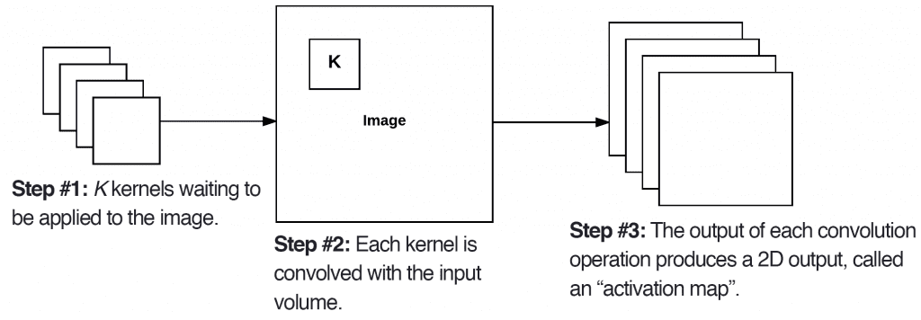
After applying all K filters to the input volume, we now have K, 2-dimensional activation maps. We then stack our K activation maps along the depth dimension of our array to form the final output volume (Figure 2).

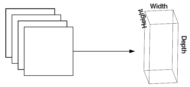
Every entry in the output volume is thus an output of a neuron that “looks” at only a small region of the input. In this manner, the network “learns” filters that activate when they see a specific type of feature at a given spatial location in the input volume. In lower layers of the network, filters may activate when they see edge-like or corner-like regions.

Then, in the deeper layers of the network, filters may activate in the presence of high-level features, such as parts of the face, the paw of a dog, the hood of a car, etc. This activation concept is as if these neurons are becoming “excited” and “activating” when they see a particular pattern in an input image.

The concept of convolving a small filter with a large(r) input volume has special meaning in Convolutional Neural Networks — specifically, the local connectivity and the receptive field of a neuron. When working with images, it’s often impractical to connect neurons in the current volume to all neurons in the previous volume — there are simply too many connections and too many weights, making it impossible to train deep networks on images with large spatial dimensions. Instead, when utilizing CNNs, we choose to connect each neuron to only a local region of the input volume — we call the size of this local region the receptive field (or simply, the variable F) of the neuron.

To make this point clear, let’s return to our CIFAR-10 dataset, where the input volume has an input size of 32×32×3. Each image thus has a width of 32 pixels, a height of 32 pixels, and a depth of 3 (one for each RGB channel). If our receptive field is of size 3×3, then each neuron in the CONV layer will connect to a 3×3 local region of the image for a total of 3×3×3 = 27 weights (remember, the depth of the filters is three because they extend through the full depth of the input image, in this case, three channels).

Now, let’s assume that the spatial dimensions of our input volume have been reduced to a smaller size, but our depth is now larger, due to utilizing more filters deeper in the network, such that the volume size is now 16×16×94. Again, if we assume a receptive field of size 3×3, then every neuron in the CONV layer will have a total of 3×3×94 = 846 connections to the input volume. Simply put, the receptive field F is the size of the filter, yielding an F×F kernel that is convolved with the input volume.

At this point, we have explained the connectivity of neurons in the input volume, but not the arrangement or size of the output volume. There are three parameters that control the size of an output volume: the depth, stride, and zero-padding size, each of which we’ll review below.

Depth

The depth of an output volume controls the number of neurons (i.e., filters) in the CONV layer that connect to a local region of the input volume. Each filter produces an activation map that “activates” in the presence of oriented edges or blobs or color.

For a given CONV layer, the depth of the activation map will be K, or simply the number of filters we are learning in the current layer. The set of filters that are “looking at” the same (x, y) location of the input is called the depth column.

Stride

Consider where we described a convolution operation as “sliding” a small matrix across a large matrix, stopping at each coordinate, computing an element-wise multiplication and sum, then storing the output. This description is similar to a sliding window (http://pyimg.co/0yizo) that slides from left-to-right and top-to-bottom across an image.

In the context of the convolution above, we only took a step of one pixel each time. In the context of CNNs, the same principle can be applied — for each step, we create a new depth column around the local region of the image, where we convolve each of the K filters with the region and store the output in a 3D volume. When creating our CONV layers we normally use a stride step size S of either S = 1 or S = 2.

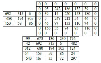
Smaller strides will lead to overlapping receptive fields and larger output volumes. Conversely, larger strides will result in less overlapping receptive fields and smaller output volumes. To make the concept of convolutional stride more concrete, consider Table 1, where we have a 5×5 input image (left) along with a 3×3 Laplacian kernel (right).

Using S = 1, our kernel slides from left-to-right and top-to-bottom, one pixel at a time, producing the following output (Table 2, left). However, if we were to apply the same operation, only this time with a stride of S = 2, we skip two pixels at a time (two pixels along the x-axis and two pixels along the y-axis), producing a smaller output volume (right).

Thus, we can see how convolution layers can be used to reduce the spatial dimensions of the input volumes simply by changing the stride of the kernel. Convolutional layers and pooling layers are the primary methods to reduce spatial input size.

Zero-padding

We need to “pad” the borders of an image to retain the original image size when applying a convolution — the same is true for filters inside of a CNN. Using zero-padding, we can “pad” our input along the borders such that our output volume size matches our input volume size. The amount of padding we apply is controlled by the parameter P.

This technique is especially critical when we start looking at deep CNN architectures that apply multiple CONV filters on top of each other. To visualize zero-padding, again refer to Table 1, where we applied a 3×3 Laplacian kernel to a 5×5 input image with a stride of S = 1.

We can see in Table 3 (left) how the output volume is smaller (3×3) than the input volume (5×5) due to the nature of the convolution operation. If we instead set P = 1, we can pad our input volume with zeros (right) to create a 7×7 volume and then apply the convolution operation, leading to an output volume size that matches the original input volume size of 5×5 (bottom).

Without zero padding, the spatial dimensions of the input volume would decrease too quickly, and we wouldn’t be able to train deep networks (as the input volumes would be too tiny to learn any useful patterns from).

Putting all these parameters together, we can compute the size of an output volume as a function of the input volume size (W, assuming the input images are square, which they nearly always are), the receptive field size F, the stride S, and the amount of zero-padding P. To construct a valid CONV layer, we need to ensure the following equation is an integer:

(1) ((W − F + 2P) / S) + 1

If it is not an integer, then the strides are set incorrectly, and the neurons cannot be tiled such that they fit across the input volume in a symmetric way.

As an example, consider the first layer of the AlexNet architecture which won the 2012 ImageNet classification challenge and is hugely responsible for the current boom of deep learning applied to image classification. Inside their paper, Krizhevsky et al. (2012) documented their CNN architecture according to Figure 3.

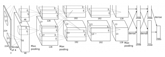
Notice how the first layer claims that the input image size is 224×224 pixels. However, this can’t possibly be correct if we apply our equation above using 11×11 filters, a stride of four, and no padding:

(2) ((224 − 11 + 2(0)) / 4) + 1 = 54.25

Which is certainly not an integer.

For novice readers just getting started in deep learning and CNNs, this small error in such a seminal paper has caused countless errors of confusion and frustration. It’s unknown why this typo occurred, but it’s likely that Krizhevsky et al. used 227×227 input images, since:

(3) ((227 − 11 + 2(0)) / 4) + 1 = 55

Errors like these are more common than you might think, so when implementing CNNs from publications, be sure to check the parameters yourself rather than simply assuming the parameters listed are correct. Due to the vast number of parameters in a CNN, it’s quite easy to make a typographical mistake when documenting an architecture (I’ve done it myself many times).

To summarize, the CONV layer in the same, elegant manner as Karpathy:

• Accepts an input volume of size W_input×H_input×D_input (the input sizes are normally square, so it’s common to see W_input = H_input).
• Requires four parameters:
  • The number of filters K (which controls the depth of the output volume).
  • The receptive field size F (the size of the K kernels used for convolution and is early always square, yielding an F×F kernel).
  • The stride S.
  • The amount of zero-padding P.

• The output of the CONV layer is then W_output×H_output×D_output, where:
  • W_output = ((W_input −F +2P) /S) +1
  • H_output = ((H_input −F +2P) / S) +1
  • D_output = K

Activation Layers

After each CONV layer in a CNN, we apply a nonlinear activation function, such as ReLU, ELU, or any of the other Leaky ReLU variants. We typically denote activation layers as RELU in network diagrams as since ReLU activations are most commonly used, we may also simply state ACT — in either case, we are making it clear that an activation function is being applied inside the network architecture.

Activation layers are not technically “layers” (due to the fact that no parameters/weights are learned inside an activation layer) and are sometimes omitted from network architecture diagrams as it’s assumed that an activation immediately follows a convolution.

In this case, authors of publications will mention which activation function they are using after each CONV layer somewhere in their paper. As an example, consider the following network architecture: INPUT => CONV => RELU => FC.

To make this diagram more concise, we could simply remove the RELU component since it’s assumed that an activation always follows a convolution: INPUT => CONV => FC. I personally do not like this and choose to explicitly include the activation layer in a network diagram to make it clear when and what activation function I am applying in the network.

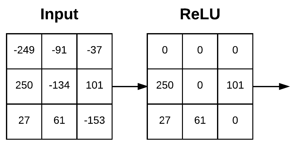
An activation layer accepts an input volume of size W_input×H_input×D_input and then applies the given activation function (Figure 4). Since the activation function is applied in an element-wise manner, the output of an activation layer is always the same as the input dimension, W_input = W_output, H_input = H_output, D_input = D_output.

Pooling Layers

There are two methods to reduce the size of an input volume — CONV layers with a stride > 1 (which we’ve already seen) and POOL layers. It is common to insert POOL layers in-between consecutive CONV layers in a CNN architectures:

INPUT => CONV => RELU => POOL => CONV => RELU => POOL => FC

The primary function of the POOL layer is to progressively reduce the spatial size (i.e., width and height) of the input volume. Doing this allows us to reduce the amount of parameters and computation in the network — pooling also helps us control overfitting.

POOL layers operate on each of the depth slices of an input independently using either the max or average function. Max pooling is typically done in the middle of the CNN architecture to reduce spatial size, whereas average pooling is normally used as the final layer of the network (e.g., GoogLeNet, SqueezeNet, ResNet), where we wish to avoid using FC layers entirely. The most common type of POOL layer is max pooling, although this trend is changing with the introduction of more exotic micro-architectures.

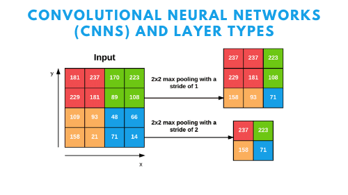
Typically we’ll use a pool size of 2×2, although deeper CNNs that use larger input images (> 200 pixels) may use a 3×3 pool size early in the network architecture. We also commonly set the stride to either S = 1 or S = 2. Figure 5 (heavily inspired by Karpathy et al.) follows an example of applying max pooling with 2×2 pool size and a stride of S = 1. Notice for every 2×2 block, we keep only the largest value, take a single step (like a sliding window), and apply the operation again — thus producing an output volume size of 3×3.

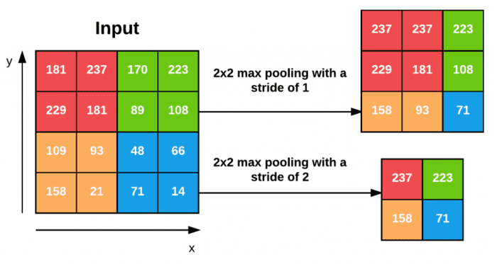
We can further decrease the size of our output volume by increasing the stride — here we apply S = 2 to the same input (Figure 5, bottom). For every 2×2 block in the input, we keep only the largest value, then take a step of two pixels, and apply the operation again. This pooling allows us to reduce the width and height by a factor of two, effectively discarding 75% of activations from the previous layer.

In summary, POOL layers Accept an input volume of size W_input×H_input×D_input. They then require two parameters:

• The receptive field size F (also called the “pool size”).
• The stride S.

Applying the POOL operation yields an output volume of size W_output×H_output×D_output, where:

• W_output = ((W_input −F) / S) +1
• H_output = ((H_input −F) / S) +1
• D_output = D_input

In practice, we tend to see two types of max pooling variations:

• Type #1: F = 3, S = 2, which is called overlapping pooling and normally applied to images/input volumes with large spatial dimensions.
• Type #2: F = 2, S = 2, which is called non-overlapping pooling. This is the most common type of pooling and is applied to images with smaller spatial dimensions.

For network architectures that accept smaller input images (in the range of 32−64 pixels) you may also see F = 2, S = 1 as well.

To POOL or CONV?

In their 2014 paper, Striving for Simplicity: The All Convolutional Net, Springenberg et al. recommend discarding the POOL layer entirely and simply relying on CONV layers with a larger stride to handle downsampling the spatial dimensions of the volume. Their work demonstrated this approach works very well on a variety of datasets, including CIFAR-10 (small images, low number of classes) and ImageNet (large input images, 1,000 classes). This trend continues with the ResNet architecture, which uses CONV layers for downsampling as well.

It’s becoming increasingly more common to not use POOL layers in the middle of the network architecture and only use average pooling at the end of the network if FC layers are to be avoided. Perhaps in the future there won’t be pooling layers in Convolutional Neural Networks — but in the meantime, it’s important that we study them, learn how they work, and apply them to our own architectures.

Fully connected Layers

Neurons in FC layers are fully connected to all activations in the previous layer, as is the standard for feedforward neural networks. FC layers are always placed at the end of the network (i.e., we don’t apply a CONV layer, then an FC layer, followed by another CONV) layer.

It’s common to use one or two FC layers prior to applying the softmax classifier, as the following (simplified) architecture demonstrates:

INPUT => CONV => RELU => POOL => CONV => RELU => POOL => FC => FC

Here, we apply two fully connected layers before our (implied) softmax classifier which will compute our final output probabilities for each class.

Batch Normalization

First introduced by Ioffe and Szegedy in their 2015 paper, Batch Normalization: Accelerating Deep Network Training by Reducing Internal Covariate Shift, batch normalization layers (or BN for short), as the name suggests, are used to normalize the activations of a given input volume before passing it into the next layer in the network.

If we consider to be our mini-batch of activations, then we can compute the normalized via the following equation:

(4)

During training, we compute the µ_β and σ_β over each mini-batch β, where:

(5)

We set ε equal to a small positive value such as 1e-7 to avoid dividing by zero. Applying this equation implies that the activations leaving a batch normalization layer will have approximately zero mean and unit variance (i.e., zero-centered).

At testing time, we replace the mini-batch µ_β and σ_β with running averages of µ_β and σ_β computed during the training process. This ensures that we can pass images through our network and still obtain accurate predictions without being biased by the µ_β and σ_β from the final mini-batch passed through the network at training time.

Batch normalization has been shown to be extremely effective at reducing the number of epochs it takes to train a neural network. Batch normalization also has the added benefit of helping “stabilize” training, allowing for a larger variety of learning rates and regularization strengths. Using batch normalization doesn’t alleviate the need to tune these parameters of course, but it will make your life easier by making learning rate and regularization less volatile and more straightforward to tune. You’ll also tend to notice lower final loss and a more stable loss curve when using batch normalization in your networks.

The biggest drawback of batch normalization is that it can actually slow down the wall time it takes to train your network (even though you’ll need fewer epochs to obtain reasonable accuracy) by 2-3x due to the computation of per-batch statistics and normalization.

That said, I recommend using batch normalization in nearly every situation as it does make a significant difference. Applying batch normalization to our network architectures can help us prevent overfitting and allows us to obtain significantly higher classification accuracy in fewer epochs compared to the same network architecture without batch normalization.

So, Where Do the Batch Normalization Layers Go?

You’ve probably noticed in my discussion of batch normalization I’ve left out exactly where in the network architecture we place the batch normalization layer. According to the original paper by Ioffe and Szegedy, they placed their batch normalization (BN) before the activation:

We add the BN transform immediately before the nonlinearity, by normalizing x = Wu + b.

Using this scheme, a network architecture utilizing batch normalization would look like this:

INPUT => CONV => BN => RELU ...

However, this view of batch normalization doesn’t make sense from a statistical point of view. In this context, a BN layer is normalizing the distribution of features coming out of a CONV layer. Some of these features may be negative, in which they will be clamped (i.e., set to zero) by a nonlinear activation function such as ReLU.

If we normalize before activation, we are essentially including the negative values inside the normalization. Our zero-centered features are then passed through the ReLU where we kill of any activations less than zero (which include features that may have not been negative before the normalization) — this layer ordering entirely defeats the purpose of applying batch normalization in the first place.

Instead, if we place the batch normalization after the ReLU we will normalize the positive valued features without statistically biasing them with features that would have otherwise not made it to the next CONV layer. In fact, François Chollet, the creator and maintainer of Keras confirms this point stating that the BN should come after the activation:

I can guarantee that recent code written by Christian [Szegedy, from the BN paper] applies relu before BN. It is still occasionally a topic of debate, though.

Szegedy

It is unclear why Ioffe and Szegedy suggested placing the BN layer before the activation in their paper, but further experiments as well as anecdotal evidence from other deep learning researchers confirm that placing the batch normalization layer after the nonlinear activation yields higher accuracy and lower loss in nearly all situations.

Placing the BN after the activation in a network architecture would look like this:

INPUT => CONV => RELU => BN ...

I can confirm that in nearly all experiments I’ve performed with CNNs, placing the BN after the RELU yields slightly higher accuracy and lower loss. That said, take note of the word “nearly” — there have been a very small number of situations where placing the BN before the activation worked better, which implies that you should default to placing the BN after the activation, but may want to dedicate (at most) one experiment to placing the BN before the activation and noting the results.

After running a few of these experiments, you’ll quickly realize that BN after the activation performs better and there are more important parameters to your network to tune to obtain higher classification accuracy.

Dropout

The last layer type we are going to discuss is dropout. Dropout is actually a form of regularization that aims to help prevent overfitting by increasing testing accuracy, perhaps at the expense of training accuracy. For each mini-batch in our training set, dropout layers, with probability p, randomly disconnect inputs from the preceding layer to the next layer in the network architecture.

Figure 6 visualizes this concept where we randomly disconnect with probability p = 0.5 the connections between two FC layers for a given mini-batch. Again, notice how half of the connections are severed for this mini-batch. After the forward and backward pass are computed for the mini-batch, we re-connect the dropped connections, and then sample another set of connections to drop.

The reason we apply dropout is to reduce overfitting by explicitly altering the network architecture at training time. Randomly dropping connections ensures that no single node in the network is responsible for “activating” when presented with a given pattern. Instead, dropout ensures there are multiple, redundant nodes that will activate when presented with similar inputs — this, in turn, helps our model to generalize.

It is most common to place dropout layers with p = 0.5 in-between FC layers of an architecture where the final FC layer is assumed to be our softmax classifier:

... CONV => RELU => POOL => FC => DO => FC => DO => FC

However, we may also apply dropout with smaller probabilities (i.e., p = 0.10−0.25) in earlier layers of the network as well (normally following a downsampling operation, either via max pooling or convolution).

Common Architectures and Training Patterns

As we have seen, Convolutional Neural Networks are made up of four primary layers: CONV, POOL, RELU, and FC. Taking these layers and stacking them together in a particular pattern yields a CNN architecture.

The CONV and FC layers (and BN) are the only layers of the network that actually learn parameters; the other layers are simply responsible for performing a given operation. Activation layers, (ACT) such as RELU and dropout aren’t technically layers, but are often included in the CNN architecture diagrams to make the operation order explicitly clear — we’ll adopt the same convention.

Layer Patterns

By far, the most common form of CNN architecture is to stack a few CONV and RELU layers, following them with a POOL operation. We repeat this sequence until the volume width and height is small, at which point we apply one or more FC layers. Therefore, we can derive the most common CNN architecture using the following pattern:

INPUT => [[CONV => RELU]*N => POOL?]*M => [FC => RELU]*K => FC

Here the * operator implies one or more and the ? indicates an optional operation.

Common choices for each repetition include:

• 0 <= N <= 3
• M >= 0
• 0 <= K <= 2

Below, we can see some examples of CNN architectures that follow this pattern:

• INPUT => FC
• INPUT => [CONV => RELU => POOL] * 2 => FC => RELU => FC
• INPUT => [CONV => RELU => CONV => RELU => POOL] * 3 => [FC => RELU] * 2 => FC

Here is an example of a very shallow CNN with only one CONV layer (N = M = K = 0):

INPUT => CONV => RELU => FC

Below is an example of an AlexNet-like CNN architecture which has multiple CONV => RELU => POOL layer sets, followed by FC layers:

INPUT => [CONV => RELU => POOL] * 2 => [CONV => RELU] * 3 => POOL =>
	[FC => RELU => DO] * 2 => SOFTMAX

For deeper network architectures, such as VGGNet, we’ll stack two (or more) layers before every POOL layer:

INPUT => [CONV => RELU] * 2 => POOL => [CONV => RELU] * 2 => POOL =>
	[CONV => RELU] * 3 => POOL => [CONV => RELU] * 3 => POOL =>
	[FC => RELU => DO] * 2 => SOFTMAX

Generally, we apply deeper network architectures when we (1) have lots of labeled training data and (2) the classification problem is sufficiently challenging. Stacking multiple CONV layers before applying a POOL layer allows the CONV layers to develop more complex features before the destructive pooling operation is performed.

There are more “exotic” network architectures that deviate from these patterns and, in turn, have created patterns of their own. Some architectures remove the POOL operation entirely, relying on CONV layers to downsample the volume — then, at the end of the network, average pooling is applied rather than FC layers to obtain the input to the softmax classifiers.

Network architectures such as GoogLeNet, ResNet, and SqueezeNet (He et al., Szegedy et al., Iandola et al.) are great examples of this pattern and demonstrate how removing FC layers leads to less parameters and faster training time.

These types of network architectures also “stack” and concatenate filters across the channel dimension: GoogLeNet applies 1×1, 3×3, and 5×5 filters and then concatenates them together across the channel dimension to learn multi-level features. Again, these architectures are considered more “exotic” and considered advanced techniques.

Rules of Thumb

I’ll review common rules of thumb when constructing your own CNNs. To start, the images presented to the input layer should be square. Using square inputs allows us to take advantage of linear algebra optimization libraries. Common input layer sizes include 32×32, 64×64, 96×96, 224×224, 227×227, and 229×229 (leaving out the number of channels for notational convenience).

Secondly, the input layer should also be divisible by two multiple times after the first CONV operation is applied. You can do this by tweaking your filter size and stride. The “divisible by two rule” enables the spatial inputs in our network to be conveniently down sampled via POOL operation in an efficient manner.

In general, your CONV layers should use smaller filter sizes such as 3×3 and 5×5. Tiny 1×1 filters are used to learn local features, but only in your more advanced network architectures. Larger filter sizes such as 7×7 and 11×11 may be used as the first CONV layer in the network (to reduce spatial input size, provided your images are sufficiently larger than > 200×200 pixels); however, after this initial CONV layer the filter size should drop dramatically, otherwise you will reduce the spatial dimensions of your volume too quickly.

You’ll also commonly use a stride of S = 1 for CONV layers, at least for smaller spatial input volumes (networks that accept larger input volumes use a stride S >= 2 in the first CONV layer to help reduce spatial dimensions). Using a stride of S = 1 enables our CONV layers to learn filters while the POOL layer is responsible for downsampling. However, keep in mind that not all network architectures follow this pattern — some architectures skip max pooling altogether and rely on the CONV stride to reduce volume size.

My personal preference is to apply zero-padding to my CONV layers to ensure the output dimension size matches the input dimension size — the only exception to this rule is if I want to purposely reduce spatial dimensions via convolution. Applying zero-padding when stacking multiple CONV layers on top of each other has also been demonstrated to increase classification accuracy in practice. Libraries such as Keras can automatically compute zero-padding for you, making it even easier to build CNN architectures.

A second personal recommendation is to use POOL layers (rather than CONV layers) to reduce the spatial dimensions of your input, at least until you become more experienced constructing your own CNN architectures. Once you reach that point, you should start experimenting with using CONV layers to reduce spatial input size and try removing max pooling layers from your architecture.

Most commonly, you’ll see max pooling applied over a 2×2 receptive field size and a stride of S = 2. You might also see a 3×3 receptive field early in the network architecture to help reduce image size. It is highly uncommon to see receptive fields larger than three since these operations are very destructive to their inputs.

Batch normalization is an expensive operation that can double or triple the amount of time it takes to train your CNN; however, I recommend using BN in nearly all situations. While BN does indeed slow down the training time, it also tends to “stabilize” training, making it easier to tune other hyperparameters (there are some exceptions, of course).

I also place the batch normalization after the activation, as has become commonplace in the deep learning community even though it goes against the original Ioffe and Szegedy paper.

Inserting BN into the common layer architectures above, they become:

• INPUT => CONV => RELU => BN => FC
• INPUT => [CONV => RELU => BN => POOL] * 2 => FC => RELU => BN => FC
• INPUT => [CONV => RELU => BN => CONV => RELU => BN => POOL] * 3 => [FC RELU => BN] * 2 => FC

You do not apply batch normalization before the softmax classifier as at this point we assume our network has learned its discriminative features earlier in the architecture.

Dropout (DO) is typically applied in between FC layers with a dropout probability of 50% — you should consider applying dropout in nearly every architecture you build. While not always performed, I also like to include dropout layers (with a very small probability, 10-25%) between POOL and CONV layers. Due to the local connectivity of CONV layers, dropout is less effective here, but I’ve often found it helpful when battling overfitting.

By keeping these rules of thumb in mind, you’ll be able to reduce your headaches when constructing CNN architectures since your CONV layers will preserve input sizes while the POOL layers take care of reducing spatial dimensions of the volumes, eventually leading to FC layers and the final output classifications.

Once you master this “traditional” method of building Convolutional Neural Networks, you should then start exploring leaving max pooling operations out entirely and using just CONV layers to reduce spatial dimensions, eventually leading to average pooling rather than an FC layer.

To download the source code to this post (and be notified when future tutorials are published here on PyImageSearch), simply enter your email address in the form below!