A few months ago, I wrote a tutorial on how to classify images using Convolutional Neural Networks (specifically, VGG16) pre-trained on the ImageNet dataset with Python and the Keras deep learning library.

The pre-trained networks inside of Keras are capable of recognizing 1,000 different object categories, similar to objects we encounter in our day-to-day lives with high accuracy.
Back then, the pre-trained ImageNet models were separate from the core Keras library, requiring us to clone a free-standing GitHub repo and then manually copy the code into our projects.
This solution worked well enough; however, since my original blog post was published, the pre-trained networks (VGG16, VGG19, ResNet50, Inception V3, and Xception) have been fully integrated into the Keras core (no need to clone down a separate repo anymore) — these implementations can be found inside the applications sub-module.
Because of this, I’ve decided to create a new, updated tutorial that demonstrates how to utilize these state-of-the-art networks in your own classification projects.
Specifically, we’ll create a special Python script that can load any of these networks using either a TensorFlow or Theano backend, and then classify your own custom input images.
To learn more about classifying images with VGGNet, ResNet, Inception, and Xception, just keep reading.
VGGNet, ResNet, Inception, and Xception with Keras
2020-06-15 Update: This blog post is now TensorFlow 2+ compatible!
In the first half of this blog post, I’ll briefly discuss the VGG, ResNet, Inception, and Xception network architectures included in the Keras library.
We’ll then create a custom Python script using Keras that can load these pre-trained network architectures from disk and classify your own input images.
Finally, we’ll review the results of these classifications on a few sample images.
State-of-the-art deep learning image classifiers in Keras
Keras ships out-of-the-box with five Convolutional Neural Networks that have been pre-trained on the ImageNet dataset:
- VGG16
- VGG19
- ResNet50
- Inception V3
- Xception
Let’s start with a overview of the ImageNet dataset and then move into a brief discussion of each network architecture.
What is ImageNet?
ImageNet is formally a project aimed at (manually) labeling and categorizing images into almost 22,000 separate object categories for the purpose of computer vision research.
However, when we hear the term “ImageNet” in the context of deep learning and Convolutional Neural Networks, we are likely referring to the ImageNet Large Scale Visual Recognition Challenge, or ILSVRC for short.
The goal of this image classification challenge is to train a model that can correctly classify an input image into 1,000 separate object categories.
Models are trained on ~1.2 million training images with another 50,000 images for validation and 100,000 images for testing.
These 1,000 image categories represent object classes that we encounter in our day-to-day lives, such as species of dogs, cats, various household objects, vehicle types, and much more. You can find the full list of object categories in the ILSVRC challenge here.
When it comes to image classification, the ImageNet challenge is the de facto benchmark for computer vision classification algorithms — and the leaderboard for this challenge has been dominated by Convolutional Neural Networks and deep learning techniques since 2012.
The state-of-the-art pre-trained networks included in the Keras core library represent some of the highest performing Convolutional Neural Networks on the ImageNet challenge over the past few years. These networks also demonstrate a strong ability to generalize to images outside the ImageNet dataset via transfer learning, such as feature extraction and fine-tuning.
VGG16 and VGG19
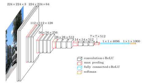
The VGG network architecture was introduced by Simonyan and Zisserman in their 2014 paper, Very Deep Convolutional Networks for Large Scale Image Recognition.
This network is characterized by its simplicity, using only 3×3 convolutional layers stacked on top of each other in increasing depth. Reducing volume size is handled by max pooling. Two fully-connected layers, each with 4,096 nodes are then followed by a softmax classifier (above).
The “16” and “19” stand for the number of weight layers in the network (columns D and E in Figure 2 below):
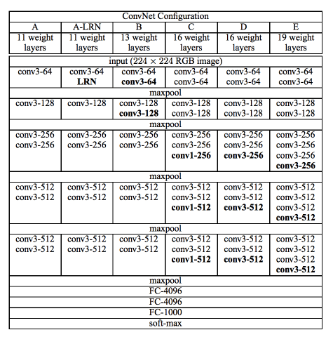
In 2014, 16 and 19 layer networks were considered very deep (although we now have the ResNet architecture which can be successfully trained at depths of 50-200 for ImageNet and over 1,000 for CIFAR-10).
Simonyan and Zisserman found training VGG16 and VGG19 challenging (specifically regarding convergence on the deeper networks), so in order to make training easier, they first trained smaller versions of VGG with less weight layers (columns A and C) first.
The smaller networks converged and were then used as initializations for the larger, deeper networks — this process is called pre-training.
While making logical sense, pre-training is a very time consuming, tedious task, requiring an entire network to be trained before it can serve as an initialization for a deeper network.
We no longer use pre-training (in most cases) and instead prefer Xaiver/Glorot initialization or MSRA initialization (sometimes called He et al. initialization from the paper, Delving Deep into Rectifiers: Surpassing Human-Level Performance on ImageNet Classification). You can read more about the importance of weight initialization and the convergence of deep neural networks inside All you need is a good init, Mishkin and Matas (2015).
Unfortunately, there are two major drawbacks with VGGNet:
- It is painfully slow to train.
- The network architecture weights themselves are quite large (in terms of disk/bandwidth).
Due to its depth and number of fully-connected nodes, VGG is over 533MB for VGG16 and 574MB for VGG19. This makes deploying VGG a tiresome task.
We still use VGG in many deep learning image classification problems; however, smaller network architectures are often more desirable (such as SqueezeNet, GoogLeNet, etc.).
ResNet
Unlike traditional sequential network architectures such as AlexNet, OverFeat, and VGG, ResNet is instead a form of “exotic architecture” that relies on micro-architecture modules (also called “network-in-network architectures”).
The term micro-architecture refers to the set of “building blocks” used to construct the network. A collection of micro-architecture building blocks (along with your standard CONV, POOL, etc. layers) leads to the macro-architecture (i.e,. the end network itself).
First introduced by He et al. in their 2015 paper, Deep Residual Learning for Image Recognition, the ResNet architecture has become a seminal work, demonstrating that extremely deep networks can be trained using standard SGD (and a reasonable initialization function) through the use of residual modules:
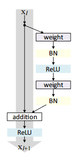
Further accuracy can be obtained by updating the residual module to use identity mappings, as demonstrated in their 2016 followup publication, Identity Mappings in Deep Residual Networks:

That said, keep in mind that the ResNet50 (as in 50 weight layers) implementation in the Keras core is based on the former 2015 paper.
Even though ResNet is much deeper than VGG16 and VGG19, the model size is actually substantially smaller due to the usage of global average pooling rather than fully-connected layers — this reduces the model size down to 102MB for ResNet50.
Inception V3
The “Inception” micro-architecture was first introduced by Szegedy et al. in their 2014 paper, Going Deeper with Convolutions:
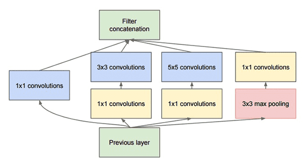
The goal of the inception module is to act as a “multi-level feature extractor” by computing 1×1, 3×3, and 5×5 convolutions within the same module of the network — the output of these filters are then stacked along the channel dimension and before being fed into the next layer in the network.
The original incarnation of this architecture was called GoogLeNet, but subsequent manifestations have simply been called Inception vN where N refers to the version number put out by Google.
The Inception V3 architecture included in the Keras core comes from the later publication by Szegedy et al., Rethinking the Inception Architecture for Computer Vision (2015) which proposes updates to the inception module to further boost ImageNet classification accuracy.
The weights for Inception V3 are smaller than both VGG and ResNet, coming in at 96MB.
Xception
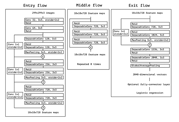
Xception was proposed by none other than François Chollet himself, the creator and chief maintainer of the Keras library.
Xception is an extension of the Inception architecture which replaces the standard Inception modules with depthwise separable convolutions.
The original publication, Xception: Deep Learning with Depthwise Separable Convolutions can be found here.
Xception sports the smallest weight serialization at only 91MB.
What about SqueezeNet?
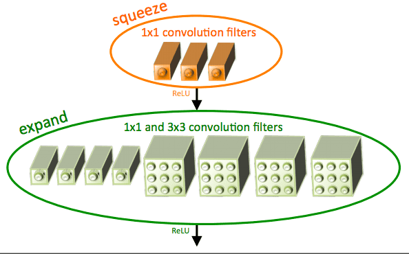
For what it’s worth, the SqueezeNet architecture can obtain AlexNet-level accuracy (~57% rank-1 and ~80% rank-5) at only 4.9MB through the usage of “fire” modules that “squeeze” and “expand”.
While leaving a small footprint, SqueezeNet can also be very tricky to train.
That said, I demonstrate how to train SqueezeNet from scratch on the ImageNet dataset inside my upcoming book, Deep Learning for Computer Vision with Python.
Configuring your development environment
To configure your system for this tutorial, I recommend following either of these tutorials:
Either tutorial will help you configure you system with all the necessary software for this blog post in a convenient Python virtual environment.
Please note that PyImageSearch does not recommend or support Windows for CV/DL projects.
Classifying images with VGGNet, ResNet, Inception, and Xception with Python and Keras
Let’s learn how to classify images with pre-trained Convolutional Neural Networks using the Keras library.
Open up a new file, name it classify_image.py , and insert the following code:
# import the necessary packages
from tensorflow.keras.applications import ResNet50
from tensorflow.keras.applications import InceptionV3
from tensorflow.keras.applications import Xception # TensorFlow ONLY
from tensorflow.keras.applications import VGG16
from tensorflow.keras.applications import VGG19
from tensorflow.keras.applications import imagenet_utils
from tensorflow.keras.applications.inception_v3 import preprocess_input
from tensorflow.keras.preprocessing.image import img_to_array
from tensorflow.keras.preprocessing.image import load_img
import numpy as np
import argparse
import cv2
Lines 2-13 import our required Python packages. As you can see, most of the packages are part of the Keras library.
Specifically, Lines 2-6 handle importing the Keras implementations of ResNet50, Inception V3, Xception, VGG16, and VGG19, respectively.
Please note that the Xception network is compatible only with the TensorFlow backend (the class will throw an error if you try to instantiate it with a Theano backend).
Line 7 gives us access to the imagenet_utils sub-module, a handy set of convenience functions that will make pre-processing our input images and decoding output classifications easier.
The remainder of the imports are other helper functions, followed by NumPy for numerical processing and cv2 for our OpenCV bindings.
Next, let’s parse our command line arguments:
# construct the argument parse and parse the arguments
ap = argparse.ArgumentParser()
ap.add_argument("-i", "--image", required=True,
	help="path to the input image")
ap.add_argument("-model", "--model", type=str, default="vgg16",
	help="name of pre-trained network to use")
args = vars(ap.parse_args())
We’ll require only a single command line argument, --image , which is the path to our input image that we wish to classify.
We’ll also accept an optional command line argument, --model , a string that specifies which pre-trained Convolutional Neural Network we would like to use — this value defaults to vgg16 for the VGG16 network architecture.
Given that we accept the name of our pre-trained network via a command line argument, we need to define a Python dictionary that maps the model names (strings) to their actual Keras classes:
# define a dictionary that maps model names to their classes
# inside Keras
MODELS = {
	"vgg16": VGG16,
	"vgg19": VGG19,
	"inception": InceptionV3,
	"xception": Xception, # TensorFlow ONLY
	"resnet": ResNet50
}

# esnure a valid model name was supplied via command line argument
if args["model"] not in MODELS.keys():
	raise AssertionError("The --model command line argument should "
		"be a key in the `MODELS` dictionary")
Lines 25-31 defines our MODELS dictionary which maps a model name string to the corresponding class.
If the --model name is not found inside MODELS , we’ll raise an AssertionError (Lines 34-36).
A Convolutional Neural Network takes an image as an input and then returns a set of probabilities corresponding to the class labels as output.
Typical input image sizes to a Convolutional Neural Network trained on ImageNet are 224×224, 227×227, 256×256, and 299×299; however, you may see other dimensions as well.
VGG16, VGG19, and ResNet all accept 224×224 input images while Inception V3 and Xception require 299×299 pixel inputs, as demonstrated by the following code block:
# initialize the input image shape (224x224 pixels) along with
# the pre-processing function (this might need to be changed
# based on which model we use to classify our image)
inputShape = (224, 224)
preprocess = imagenet_utils.preprocess_input

# if we are using the InceptionV3 or Xception networks, then we
# need to set the input shape to (299x299) [rather than (224x224)]
# and use a different image pre-processing function
if args["model"] in ("inception", "xception"):
	inputShape = (299, 299)
	preprocess = preprocess_input
Here we initialize our inputShape to be 224×224 pixels. We also initialize our preprocess function to be the standard preprocess_input from Keras (which performs mean subtraction).
However, if we are using Inception or Xception, we need to set the inputShape to 299×299 pixels, followed by updating preprocess to use a separate pre-processing function that performs a different type of scaling.
The next step is to load our pre-trained network architecture weights from disk and instantiate our model:
# load our the network weights from disk (NOTE: if this is the
# first time you are running this script for a given network, the
# weights will need to be downloaded first -- depending on which
# network you are using, the weights can be 90-575MB, so be
# patient; the weights will be cached and subsequent runs of this
# script will be *much* faster)
print("[INFO] loading {}...".format(args["model"]))
Network = MODELS[args["model"]]
model = Network(weights="imagenet")
Line 58 uses the MODELS dictionary along with the --model command line argument to grab the correct Network class.
The Convolutional Neural Network is then instantiated on Line 59 using the pre-trained ImageNet weights;
Note: Weights for VGG16 and VGG19 are > 500MB. ResNet weights are ~100MB, while Inception and Xception weights are between 90-100MB. If this is the first time you are running this script for a given network, these weights will be (automatically) downloaded and cached to your local disk. Depending on your internet speed, this may take awhile. However, once the weights are downloaded, they will not need to be downloaded again, allowing subsequent runs of classify_image.py to be much faster.
Our network is now loaded and ready to classify an image — we just need to prepare this image for classification:
# load the input image using the Keras helper utility while ensuring
# the image is resized to `inputShape`, the required input dimensions
# for the ImageNet pre-trained network
print("[INFO] loading and pre-processing image...")
image = load_img(args["image"], target_size=inputShape)
image = img_to_array(image)

# our input image is now represented as a NumPy array of shape
# (inputShape[0], inputShape[1], 3) however we need to expand the
# dimension by making the shape (1, inputShape[0], inputShape[1], 3)
# so we can pass it through the network
image = np.expand_dims(image, axis=0)

# pre-process the image using the appropriate function based on the
# model that has been loaded (i.e., mean subtraction, scaling, etc.)
image = preprocess(image)
Line 65 loads our input image from disk using the supplied inputShape to resize the width and height of the image.
Line 66 converts the image from a PIL/Pillow instance to a NumPy array.
Our input image is now represented as a NumPy array with the shape (inputShape[0], inputShape[1], 3) .
However, we typically train/classify images in batches with Convolutional Neural Networks, so we need to add an extra dimension to the array via np.expand_dims on Line 72.
After calling np.expand_dims the image has the shape (1, inputShape[0], inputShape[1], 3) . Forgetting to add this extra dimension will result in an error when you call .predict of the model .
Lastly, Line 76 calls the appropriate pre-processing function to perform mean subtraction/scaling.
We are now ready to pass our image through the network and obtain the output classifications:
# classify the image
print("[INFO] classifying image with '{}'...".format(args["model"]))
preds = model.predict(image)
P = imagenet_utils.decode_predictions(preds)

# loop over the predictions and display the rank-5 predictions +
# probabilities to our terminal
for (i, (imagenetID, label, prob)) in enumerate(P[0]):
	print("{}. {}: {:.2f}%".format(i + 1, label, prob * 100))
A call to .predict on Line 80 returns the predictions from the Convolutional Neural Network.
Given these predictions, we pass them into the ImageNet utility function .decode_predictions to give us a list of ImageNet class label IDs, “human-readable” labels, and the probability associated with the labels.
The top-5 predictions (i.e., the labels with the largest probabilities) are then printed to our terminal on Lines 85 and 86.
The last thing we’ll do here before we close out our example is load our input image from disk via OpenCV, draw the #1 prediction on the image, and finally display the image to our screen:
# load the image via OpenCV, draw the top prediction on the image,
# and display the image to our screen
orig = cv2.imread(args["image"])
(imagenetID, label, prob) = P[0][0]
cv2.putText(orig, "Label: {}, {:.2f}%".format(label, prob * 100),
	(10, 30), cv2.FONT_HERSHEY_SIMPLEX, 0.8, (0, 0, 255), 2)
cv2.imshow("Classification", orig)
cv2.waitKey(0)
To see our pre-trained ImageNet networks in action, take a look at the next section.
VGGNet, ResNet, Inception, and Xception classification results
All updated examples in this blog post were gathered TensorFlow 2.2. Previously this blog post used Keras >= 2.0 and a TensorFlow backend (when they were separate packages) and was also tested with the Theano backend and confirmed that the implementation will work with Theano as well.
Once you have TensorFlow/Theano and Keras installed, make sure you download the source code + example images to this blog post using the “Downloads” section at the bottom of the tutorial.
From there, let’s try classifying an image with VGG16:
$ python classify_image.py --image images/soccer_ball.jpg --model vgg16
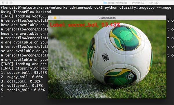
Taking a look at the output, we can see VGG16 correctly classified the image as “soccer ball” with 93.43% accuracy.
To use VGG19, we simply need to change the --model command line argument:
$ python classify_image.py --image images/bmw.png --model vgg19
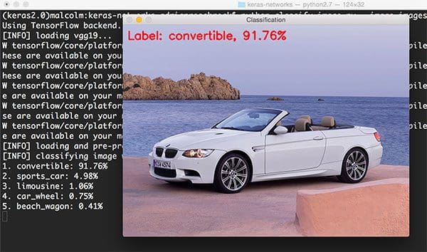
VGG19 is able to correctly classify the the input image as “convertible” with a probability of 91.76%. However, take a look at the other top-5 predictions: sports car with 4.98% probability (which the car is), limousine at 1.06% (incorrect, but still reasonable), and “car wheel” at 0.75% (also technically correct since there are car wheels in the image).
We can see similar levels of top-5 accuracy in the following example where we use the pre-trained ResNet architecture:
$ python classify_image.py --image images/clint_eastwood.jpg --model resnet
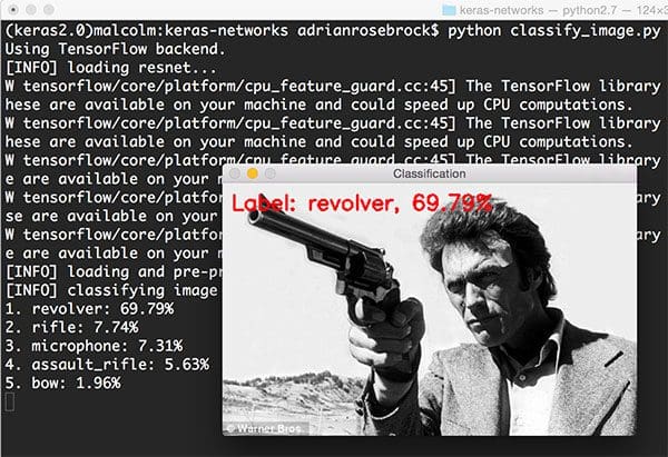
ResNet correctly classifies this image of Clint Eastwood holding a gun as “revolver” with 69.79% accuracy. It’s also interesting to see “rifle” at 7.74% and “assault rifle” at 5.63% included in the top-5 predictions as well. Given the viewing angle of the revolver and the substantial length of the barrel (for a handgun) it’s easy to see how a Convolutional Neural Network would also return higher probabilities for a rifle as well.
This next example attempts to classify the species of dog using ResNet:
$ python classify_image.py --image images/jemma.png --model resnet
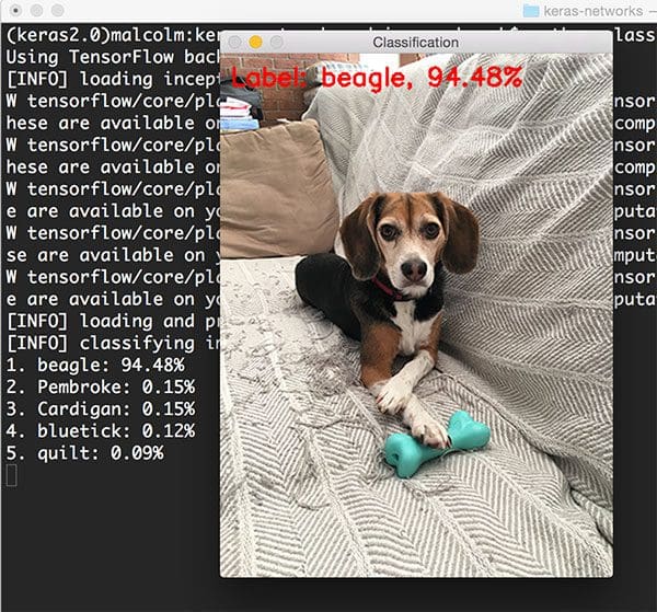
The species of dog is correctly identified as “beagle” with 94.48% confidence.
I then tried classifying the following image of Johnny Depp from the Pirates of the Caribbean franchise:
$ python classify_image.py --image images/boat.png --model inception
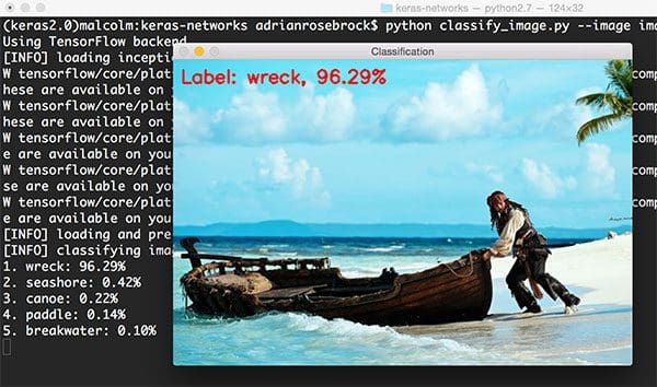
While there is indeed a “boat” class in ImageNet, it’s interesting to see that the Inception network was able to correctly identify the scene as a “(ship) wreck” with 96.29% probability. All other predicted labels, including “seashore”, “canoe”, “paddle”, and “breakwater” are all relevant, and in some cases absolutely correct as well.
For another example of the Inception network in action, I took a photo of the couch sitting in my office:
$ python classify_image.py --image images/office.png --model inception
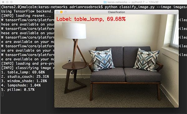
Inception correctly predicts there is a “table lamp” in the image with 69.68% confidence. The other top-5 predictions are also dead-on, including a “studio couch”, “window shade” (far right of the image, barely even noticeable), “lampshade”, and “pillow”.
In the context above, Inception wasn’t even used as an object detector, but it was still able to classify all parts of the image within its top-5 predictions. It’s no wonder that Convolutional Neural Networks make for excellent object detectors!
Moving on to Xception:
$ python classify_image.py --image images/scotch.png --model xception
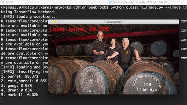
Here we have an image of scotch barrels, specifically my favorite scotch, Lagavulin. Xception correctly classifies this image as “barrels”.
This last example was classified using VGG16:
$ python classify_image.py --image images/tv.png --model vgg16
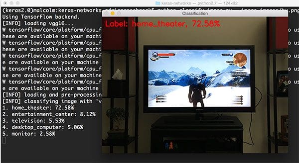
The image itself was captured a few months ago as I was finishing up The Witcher III: The Wild Hunt (easily in my top-3 favorite games of all time). The first prediction by VGG16 is “home theatre” — a reasonable prediction given that there is a “television/monitor” in the top-5 predictions as well.
As you can see from the examples in this blog post, networks pre-trained on the ImageNet dataset are capable of recognizing a variety of common day-to-day objects. I hope that you can use this code in your own projects!
What's next? We recommend PyImageSearch University.
86+ total classes • 115+ hours hours of on-demand code walkthrough videos • Last updated: April 2026
★★★★★ 4.84 (128 Ratings) • 16,000+ Students Enrolled
I strongly believe that if you had the right teacher you could master computer vision and deep learning.
Do you think learning computer vision and deep learning has to be time-consuming, overwhelming, and complicated? Or has to involve complex mathematics and equations? Or requires a degree in computer science?
That’s not the case.
All you need to master computer vision and deep learning is for someone to explain things to you in simple, intuitive terms. And that’s exactly what I do. My mission is to change education and how complex Artificial Intelligence topics are taught.
If you're serious about learning computer vision, your next stop should be PyImageSearch University, the most comprehensive computer vision, deep learning, and OpenCV course online today. Here you’ll learn how to successfully and confidently apply computer vision to your work, research, and projects. Join me in computer vision mastery.
Inside PyImageSearch University you'll find:
- ✓ 86+ courses on essential computer vision, deep learning, and OpenCV topics
- ✓ 86 Certificates of Completion
- ✓ 115+ hours hours of on-demand video
- ✓ Brand new courses released regularly, ensuring you can keep up with state-of-the-art techniques
- ✓ Pre-configured Jupyter Notebooks in Google Colab
- ✓ Run all code examples in your web browser — works on Windows, macOS, and Linux (no dev environment configuration required!)
- ✓ Access to centralized code repos for all 540+ tutorials on PyImageSearch
- ✓ Easy one-click downloads for code, datasets, pre-trained models, etc.
- ✓ Access on mobile, laptop, desktop, etc.
Summary
In today’s blog post we reviewed the five Convolutional Neural Networks pre-trained on the ImageNet dataset inside the Keras library:
- VGG16
- VGG19
- ResNet50
- Inception V3
- Xception
I then demonstrated how to use each of these architectures to classify your own input images using the Keras library and the Python programming language.
If you are interested in learning more about deep learning and Convolutional Neural Networks (and how to train your own networks from scratch), be sure to take a look at my book, Deep Learning for Computer Vision with Python, available for order now.

Download the Source Code and FREE 17-page Resource Guide
Enter your email address below to get a .zip of the code and a FREE 17-page Resource Guide on Computer Vision, OpenCV, and Deep Learning. Inside you'll find my hand-picked tutorials, books, courses, and libraries to help you master CV and DL!

