The Christmas season holds a special place in my heart.
Not because I’m particularly religious or spiritual. Not because I enjoy cold weather. And certainly not because I relish the taste of eggnog (the consistency alone makes my stomach turn).
Instead, Christmas means a lot to me because of my dad.
As I mentioned in a post a few weeks ago, I had a particularly rough childhood. There was a lot of mental illness in my family. I had to grow up fast in that environment and there were times when I missed out on the innocence of being a kid and living in the moment.
But somehow, through all that struggle, my dad made Christmas a glowing beacon of happiness.
Perhaps one of my favorite memories as a kid was when I was in kindergarten (5-6 years old). I had just gotten off the bus, book bag in hand.
I was walking down our long, curvy driveway where at the bottom of the hill I saw my dad laying out Christmas lights which would later decorate our house, bushes, and trees, transforming our home into a Christmas wonderland.
I took off like a rocket, carelessly running down the driveway (as only a child can), unzipped winter coat billowing behind me as I ran, shouting:
“Wait for me, dad!”
I didn’t want to miss out on the decorating festivities.
For the next few hours, my dad patiently helped me untangle the knotted ball of Christmas lights, lay them out, and then watched as I haphazardly threw the lights over the bushes and trees (that were many times my size), ruining any methodical, well-planned decorating blueprint he had so tirelessly designed.
Once I was finished he smiled proudly. He didn’t need any words. His smile confessed that my decorating was the best he had ever seen.
This is just one example of the many, many times my dad made Christmas special for me (despite what else may have been going on in the family).
He probably didn’t even know he was crafting a lifelong memory in my mind — he just wanted to make me happy.
Each year, when Christmas rolls around, I try to slow down, reduce stress, and enjoy the time of year.
Without my dad, I wouldn’t be where I am today — and I certainly wouldn’t have made it through my childhood.
In honor of the Christmas season, I’d like to dedicate this blog post to my dad.
Even if you’re busy, don’t have the time, or simply don’t care about deep learning (the subject matter of today’s tutorial), slow down and give this blog post a read, if for nothing else than for my dad.
I hope you enjoy it.
Image classification with Keras and deep learning
2020-05-13 Update: This blog post is now TensorFlow 2+ compatible!
This blog post is part two in our three-part series of building a Not Santa deep learning classifier (i.e., a deep learning model that can recognize if Santa Claus is in an image or not):
- Part 1: Deep learning + Google Images for training data
- Part 2: Training a Santa/Not Santa detector using deep learning (this post)
- Part 3: Deploying a Santa/Not Santa deep learning detector to the Raspberry Pi (next week’s post)
In the first part of this tutorial, we’ll examine our “Santa” and “Not Santa” datasets.
Together, these images will enable us to train a Convolutional Neural Network using Python and Keras to detect if Santa is in an image.
Once we’ve explored our training images, we’ll move on to training the seminal LeNet architecture. We’ll use a smaller network architecture to ensure readers without expensive GPUs can still follow along with this tutorial. This will also ensure beginners can understand the fundamentals of deep learning with Convolutional Neural Networks with Keras and Python.
Finally, we’ll evaluate our Not Santa model on a series of images, then discuss a few limitations to our approach (and how to further extend it).
Our “Santa” and “Not Santa” dataset
In order to train our Not Santa deep learning model, we require two sets of images:
- Images containing Santa (“Santa”).
- Images that do not contain Santa (“Not Santa”).
Last week we used our Google Images hack to quickly grab training images for deep learning networks.
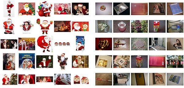
In this case, we can see a sample of the 461 images containing Santa gathered using the technique (Figure 1, left).
I then randomly sampled 461 images that do not contain Santa (Figure 1, right) from the UKBench dataset, a collection of ~10,000 images used for building and evaluating Content-based Image Retrieval (CBIR) systems (i.e., image search engines).
Used together, these two image sets will enable us to train our Not Santa deep learning model.
Configuring your development environment
To configure your system for this tutorial, I first recommend following either of these tutorials:
Either tutorial will help you configure your system with all the necessary software for this blog post in a convenient Python virtual environment.
Please note that PyImageSearch does not recommend or support Windows for CV/DL projects.
Your first image classifier with Convolutional Neural Networks and Keras

The LetNet architecture is an excellent “first image classifier” for Convolutional Neural Networks. Originally designed for classifying handwritten digits, we can easily extend it to other types of images as well.
This tutorial is meant to be an introduction to image classification using deep learning, Keras, and Python so I will not be discussing the inner workings of each layer. If you are interested in taking a deep dive into deep learning, please take a look at my book, Deep Learning for Computer Vision with Python, where I discuss deep learning in detail (and with lots of code + practical, hands-on implementations as well).
Let’s go ahead and define the network architecture. Open up a new file name it lenet.py , and insert the following code:
Note: You’ll want to use the “Downloads” section of this post to download the source code + example images before running the code. I’ve included the code below as a matter of completeness, but you’ll want to ensure your directory structure matches mine.
# import the necessary packages
from tensorflow.keras.models import Sequential
from tensorflow.keras.layers import Conv2D
from tensorflow.keras.layers import MaxPooling2D
from tensorflow.keras.layers import Activation
from tensorflow.keras.layers import Flatten
from tensorflow.keras.layers import Dense
from tensorflow.keras import backend as K

class LeNet:
	@staticmethod
	def build(width, height, depth, classes):
		# initialize the model
		model = Sequential()
		inputShape = (height, width, depth)

		# if we are using "channels first", update the input shape
		if K.image_data_format() == "channels_first":
			inputShape = (depth, height, width)
Lines 2-8 handle importing our required Python packages. The Conv2D class is responsible for performing convolution. We can use the MaxPooling2D class for max-pooling operations. As the name suggests, the Activation class applies a particular activation function. When we are ready to Flatten our network topology into fully connected, Dense layer(s) we can use the respective class names.
The LeNet class is defined on Line 10 followed by the build method on Line 12. Whenever I defined a new Convolutional Neural Network architecture I like to:
- Place it in its own class (for namespace and organizational purposes)
- Create a static
buildfunction that builds the architecture itself
The build method, as the name suggests, takes a number of parameters, each of which I discuss below:
width: The width of our input imagesheight: The height of the input imagesdepth: The number of channels in our input images (1for grayscale single channel images,3for standard RGB images which we’ll be using in this tutorial)classes: The total number of classes we want to recognize (in this case, two)
We define our model on Line 14. We use the Sequential class since we will be sequentially adding layers to the model .
Line 15 initializes our inputShape using channels last ordering (the default for TensorFlow). If you are using Theano (or any other backend to Keras that assumes channels first ordering), Lines 18 and 19 properly update the inputShape .
Now that we have initialized our model, we can start adding layers to it:
		# first set of CONV => RELU => POOL layers
		model.add(Conv2D(20, (5, 5), padding="same",
			input_shape=inputShape))
		model.add(Activation("relu"))
		model.add(MaxPooling2D(pool_size=(2, 2), strides=(2, 2)))
Lines 21-25 creates our first set of CONV => RELU => POOL layers.
The CONV layer will learn 20 convolution filters, each of which are 5×5.
We then apply a ReLU activation function followed by 2×2 max-pooling in both the x and y direction with a stride of two. To visualize this operation, consider a sliding window that “slides” across the activation volume, taking the max operation over each region, while taking a step of two pixels in both the horizontal and vertical direction.
Let’s define our second set of CONV => RELU => POOL layers:
		# second set of CONV => RELU => POOL layers
		model.add(Conv2D(50, (5, 5), padding="same"))
		model.add(Activation("relu"))
		model.add(MaxPooling2D(pool_size=(2, 2), strides=(2, 2)))
This time we are learning 50 convolutional filters rather than the 20 convolutional filters as in the previous layer set. It’s common to see the number of CONV filters learned increase the deeper we go in the network architecture.
Our final code block handles flattening out the volume into a set of fully-connected layers:
		# first (and only) set of FC => RELU layers
		model.add(Flatten())
		model.add(Dense(500))
		model.add(Activation("relu"))

		# softmax classifier
		model.add(Dense(classes))
		model.add(Activation("softmax"))

		# return the constructed network architecture
		return model
On Line 33, we take the output of the preceding MaxPooling2D layer and flatten it into a single vector. This operation allows us to apply our dense/fully-connected layers.
Our fully-connected layer contains 500 nodes (Line 34) which we then pass through another nonlinear ReLU activation.
Line 38 defines another fully-connected layer, but this one is special — the number of nodes is equal to the number of classes (i.e., the classes we want to recognize).
This Dense layer is then fed into our softmax classifier which will yield the probability for each class.
Finally, Line 42 returns our fully constructed deep learning + Keras image classifier to the calling function.
Training our Convolutional Neural Network image classifier with Keras
Let’s go ahead and get started training our image classifier using deep learning, Keras, and Python.
Note: Be sure to scroll down to the “Downloads” section to grab the code + training images. This will enable you to follow along with the post and then train your image classifier using the dataset we have put together for you.
Open up a new file, name it train_network.py , and insert the following code (or simply follow along with the code download):
# set the matplotlib backend so figures can be saved in the background
import matplotlib
matplotlib.use("Agg")

# import the necessary packages
from tensorflow.keras.preprocessing.image import ImageDataGenerator
from tensorflow.keras.optimizers import Adam
from sklearn.model_selection import train_test_split
from tensorflow.keras.preprocessing.image import img_to_array
from tensorflow.keras.utils import to_categorical
from pyimagesearch.lenet import LeNet
from imutils import paths
import matplotlib.pyplot as plt
import numpy as np
import argparse
import random
import cv2
import os
On Lines 2-18, we import required packages. These packages enable us to:
- Load our image dataset from disk
- Pre-process the images
- Instantiate our Convolutional Neural Network
- Train our image classifier
Notice that on Line 3 we set the matplotlib backend to "Agg" so that we can save the plot to disk in the background. This is important if you are using a headless server to train your network (e.g., an Azure, AWS, or other cloud instance).
From there, we parse command line arguments:
# construct the argument parser and parse the arguments
ap = argparse.ArgumentParser()
ap.add_argument("-d", "--dataset", required=True,
  help="path to input dataset")
ap.add_argument("-m", "--model", required=True,
  help="path to output model")
ap.add_argument("-p", "--plot", type=str, default="plot.png",
  help="path to output loss/accuracy plot")
args = vars(ap.parse_args())
Here we have two required command line arguments, --dataset and --model , as well as an optional path to our accuracy/loss chart, --plot .
The --dataset switch should point to the directory containing the images we will be training our image classifier on (i.e., the “Santa” and “Not Santa” images) while the --model switch controls where we will save our serialized image classifier after it has been trained. If --plot is left unspecified, it will default to plot.png in this directory if unspecified.
Next, we’ll set some training variables, initialize lists, and gather paths to images:
# initialize the number of epochs to train for, initia learning rate,
# and batch size
EPOCHS = 25
INIT_LR = 1e-3
BS = 32

# initialize the data and labels
print("[INFO] loading images...")
data = []
labels = []

# grab the image paths and randomly shuffle them
imagePaths = sorted(list(paths.list_images(args["dataset"])))
random.seed(42)
random.shuffle(imagePaths)
On Lines 32-34, we define the number of training epochs, initial learning rate, and batch size.
Then we initialize data and label lists (Lines 38 and 39). These lists will be responsible for storing the images we load from disk along with their respective class labels.
From there we grab the paths to our input images followed by shuffling them (Lines 42-44).
Now let’s pre-process the images:
# loop over the input images
for imagePath in imagePaths:
	# load the image, pre-process it, and store it in the data list
	image = cv2.imread(imagePath)
	image = cv2.resize(image, (28, 28))
	image = img_to_array(image)
	data.append(image)

	# extract the class label from the image path and update the
	# labels list
	label = imagePath.split(os.path.sep)[-2]
	label = 1 if label == "santa" else 0
	labels.append(label)
This loop simply loads and resizes each image to a fixed 28×28 pixels (the spatial dimensions required for LeNet), and appends the image array to the data list (Lines 49-52) followed by extracting the class label from the imagePath on Lines 56-58.
We are able to perform this class label extraction since our dataset directory structure is organized in the following fashion:
|--- images
|    |--- not_santa
|    |    |--- 00000000.jpg
|    |    |--- 00000001.jpg
...
|    |    |--- 00000460.jpg
|    |--- santa
|    |    |--- 00000000.jpg
|    |    |--- 00000001.jpg
...
|    |    |--- 00000460.jpg
|--- pyimagesearch
|    |--- __init__.py
|    |--- lenet.py
|    |    |--- __init__.py
|    |    |--- networks
|    |    |    |--- __init__.py
|    |    |    |--- lenet.py
|--- test_network.py
|--- train_network.py
Therefore, an example imagePath would be:
images/santa/00000384.jpg
After extracting the label from the imagePath , the result is:
santa
I prefer organizing deep learning image datasets in this manner as it allows us to efficiently organize our dataset and parse out class labels without having to use a separate index/lookup file.
Next, we’ll scale images and create the training and testing splits:
# scale the raw pixel intensities to the range [0, 1]
data = np.array(data, dtype="float") / 255.0
labels = np.array(labels)

# partition the data into training and testing splits using 75% of
# the data for training and the remaining 25% for testing
(trainX, testX, trainY, testY) = train_test_split(data,
	labels, test_size=0.25, random_state=42)

# convert the labels from integers to vectors
trainY = to_categorical(trainY, num_classes=2)
testY = to_categorical(testY, num_classes=2)
On Line 61, we further pre-process our input data by scaling the data points from [0, 255] (the minimum and maximum RGB values of the image) to the range [0, 1].
We then perform a training/testing split on the data using 75% of the images for training and 25% for testing (Lines 66 and 67). This is a typical split for this amount of data.
We also convert labels to vectors using one-hot encoding — this is handled on Lines 70 and 71.
Subsequently, we’ll perform some data augmentation, enabling us to generate “additional” training data by randomly transforming the input images using the parameters below:
# construct the image generator for data augmentation
aug = ImageDataGenerator(rotation_range=30, width_shift_range=0.1,
	height_shift_range=0.1, shear_range=0.2, zoom_range=0.2,
	horizontal_flip=True, fill_mode="nearest")
Data augmentation is covered in depth in the Practitioner Bundle of my new book, Deep Learning for Computer Vision with Python.
Essentially Lines 74-76 create an image generator object which performs random rotations, shifts, flips, crops, and sheers on our image dataset. This allows us to use a smaller dataset and still achieve high results.
Let’s move on to training our image classifier using deep learning and Keras.
# initialize the model
print("[INFO] compiling model...")
model = LeNet.build(width=28, height=28, depth=3, classes=2)
opt = Adam(lr=INIT_LR, decay=INIT_LR / EPOCHS)
model.compile(loss="binary_crossentropy", optimizer=opt,
	metrics=["accuracy"])

# train the network
print("[INFO] training network...")
H = model.fit(x=aug.flow(trainX, trainY, batch_size=BS),
	validation_data=(testX, testY), steps_per_epoch=len(trainX) // BS,
	epochs=EPOCHS, verbose=1)

# save the model to disk
print("[INFO] serializing network...")
model.save(args["model"], save_format="h5")
We’ve elected to use LeNet for this project for two reasons:
- LeNet is a small Convolutional Neural Network that is easy for beginners to understand
- We can easily train LeNet on our Santa/Not Santa dataset without having to use a GPU
- If you want to study deep learning in more depth (including ResNet, GoogLeNet, SqueezeNet, and others) please take a look at my book, Deep Learning for Computer Vision with Python.
We build our LeNet model along with the Adam optimizer on Lines 80-83. Since this is a two-class classification problem we’ll want to use binary cross-entropy as our loss function. If you are performing classification with > 2 classes, be sure to swap out the loss for categorical_crossentropy.
Training our network is initiated on Lines 87-89 where we call model.fit, supplying our data augmentation object, training/testing data, and the number of epochs we wish to train for.
2020-05-13 Update: Formerly, TensorFlow/Keras required use of a method called fit_generator in order to accomplish data augmentation. Now, the fit, method can handle data augmentation as well, making for more-consistent code. Be sure to check out my articles about fit and fit generator as well as data augmentation.
Line 93 handles serializing the model to disk so we later use our image classification without having to retrain it.
Finally, let’s plot the results and see how our deep learning image classifier performed:
# plot the training loss and accuracy
plt.style.use("ggplot")
plt.figure()
N = EPOCHS
plt.plot(np.arange(0, N), H.history["loss"], label="train_loss")
plt.plot(np.arange(0, N), H.history["val_loss"], label="val_loss")
plt.plot(np.arange(0, N), H.history["accuracy"], label="train_acc")
plt.plot(np.arange(0, N), H.history["val_accuracy"], label="val_acc")
plt.title("Training Loss and Accuracy on Santa/Not Santa")
plt.xlabel("Epoch #")
plt.ylabel("Loss/Accuracy")
plt.legend(loc="lower left")
plt.savefig(args["plot"])
2020-05-13 Update: In order for this plotting snippet to be TensorFlow 2+ compatible the H.history dictionary keys are updated to fully spell out “accuracy” sans “acc” (i.e., H.history["val_accuracy"] and H.history["accuracy"]). It is semi-confusing that “val” is not spelled out as “validation”; we have to learn to love and live with the API and always remember that it is a work in progress that many developers around the world contribute to.
Using matplotlib, we build our plot and save the plot to disk using the --plot command line argument which contains the path + filename.
To train the Not Santa network (after using the “Downloads” section of this blog post to download the code + images), open up a terminal and execute the following command:
$ python train_network.py --dataset images --model santa_not_santa.model
Using TensorFlow backend.
[INFO] loading images...
[INFO] compiling model...
[INFO] training network...
Train for 21 steps, validate on 231 samples
Epoch 1/25
 1/21 [>.............................] - ETA: 11s - loss: 0.6757 - accuracy: 0.7368
21/21 [==============================] - 1s 43ms/step - loss: 0.7833 - accuracy: 0.4947 - val_loss: 0.5988 - val_accuracy: 0.5022
Epoch 2/25
21/21 [==============================] - 0s 21ms/step - loss: 0.5619 - accuracy: 0.6783 - val_loss: 0.4819 - val_accuracy: 0.7143
Epoch 3/25
21/21 [==============================] - 0s 21ms/step - loss: 0.4472 - accuracy: 0.8194 - val_loss: 0.4558 - val_accuracy: 0.7879
...
Epoch 23/25
21/21 [==============================] - 0s 23ms/step - loss: 0.1123 - accuracy: 0.9575 - val_loss: 0.2152 - val_accuracy: 0.9394
Epoch 24/25
21/21 [==============================] - 0s 23ms/step - loss: 0.1206 - accuracy: 0.9484 - val_loss: 0.4427 - val_accuracy: 0.8615
Epoch 25/25
21/21 [==============================] - 1s 25ms/step - loss: 0.1448 - accuracy: 0.9469 - val_loss: 0.1682 - val_accuracy: 0.9524
[INFO] serializing network...
As you can see, the network trained for 25 epochs and we achieved high accuracy (95.24% testing accuracy) and low loss that follows the training loss, as is apparent from the plot below:

Evaluating our Convolutional Neural Network image classifier
The next step is to evaluate our Not Santa model on example images not part of the training/testing splits.
Open up a new file, name it test_network.py , and let’s get started:
# import the necessary packages
from tensorflow.keras.preprocessing.image import img_to_array
from tensorflow.keras.models import load_model
import numpy as np
import argparse
import imutils
import cv2
On Lines 2-7 we import our required packages. Take special notice of the load_model method — this function will enable us to load our serialized Convolutional Neural Network (i.e., the one we just trained in the previous section) from disk.
Next, we’ll parse our command line arguments:
# construct the argument parser and parse the arguments
ap = argparse.ArgumentParser()
ap.add_argument("-m", "--model", required=True,
	help="path to trained model model")
ap.add_argument("-i", "--image", required=True,
	help="path to input image")
args = vars(ap.parse_args())
We require two command line arguments: our --model and an input --image (i.e., the image we are going to classify).
From there, we’ll load the image and pre-process it:
# load the image
image = cv2.imread(args["image"])
orig = image.copy()

# pre-process the image for classification
image = cv2.resize(image, (28, 28))
image = image.astype("float") / 255.0
image = img_to_array(image)
image = np.expand_dims(image, axis=0)
We load the image and make a copy of it on Lines 18 and 19. The copy allows us to later recall the original image and put our label on it.
Lines 22-25 handle scaling our image to the range [0, 1], converting it to an array, and adding an extra dimension (Lines 22-25).
As I explain in my book, Deep Learning for Computer Vision with Python, we train/classify images in batches with CNNs. Adding an extra dimension to the array via np.expand_dims allows our image to have the shape (1, width, height, 3) , assuming channels last ordering.
If we forget to add the dimension, it will result in an error when we call model.predict down the line.
From there we’ll load the Not Santa image classifier model and make a prediction:
# load the trained convolutional neural network
print("[INFO] loading network...")
model = load_model(args["model"])

# classify the input image
(notSanta, santa) = model.predict(image)[0]
This block is pretty self-explanatory, but since this is where the heavy lifting of this script is performed, let’s take a second and understand what’s going on under the hood.
We load the Not Santa model on Line 29 followed by making a prediction on Line 32.
And finally, we’ll use our prediction to draw on the orig image copy and display it to the screen:
# build the label
label = "Santa" if santa > notSanta else "Not Santa"
proba = santa if santa > notSanta else notSanta
label = "{}: {:.2f}%".format(label, proba * 100)

# draw the label on the image
output = imutils.resize(orig, width=400)
cv2.putText(output, label, (10, 25),  cv2.FONT_HERSHEY_SIMPLEX,
	0.7, (0, 255, 0), 2)

# show the output image
cv2.imshow("Output", output)
cv2.waitKey(0)
We build the label (either “Santa” or “Not Santa”) on Line 35 and then choose the corresponding probability value on Line 36.
The label and proba are used on Line 37 to build the label text to show at the image as you’ll see in the top left corner of the output images below.
We resize the images to a standard width to ensure they will fit on our screen, and then put the label text on the image (Lines 40-42).
Finally, on Lines 45, we display the output image until a key has been pressed (Line 46).
Let’s give our Not Santa deep learning network a try:
$ python test_network.py --model santa_not_santa.model \
	--image examples/santa_01.png

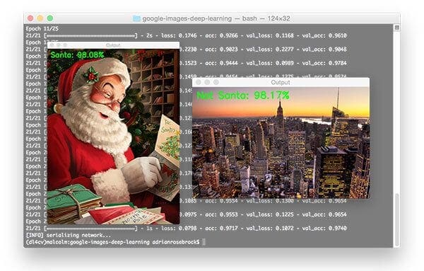
By golly! Our software thinks it is good ole’ St. Nick, so it really must be him!
Let’s try another image:
$ python test_network.py --model santa_not_santa.model \
	--image examples/santa_02.png
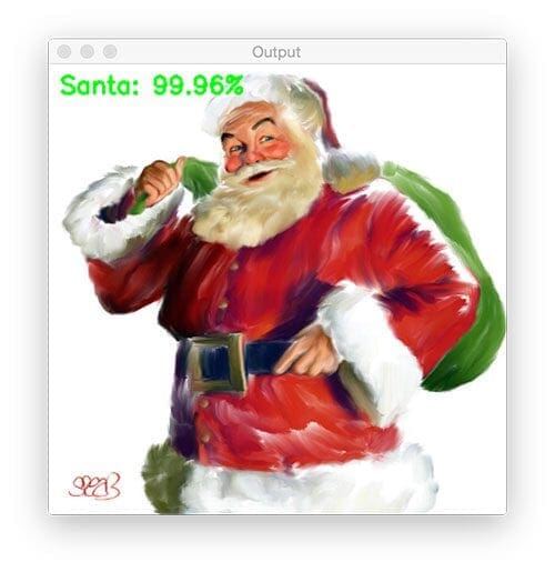
Santa is correctly detected by the Not Santa detector and it looks like he’s happy to be delivering some toys!
Now, let’s perform image classification on an image that does not contain Santa:
$ python test_network.py --model santa_not_santa.model \
	--image examples/manhattan.png
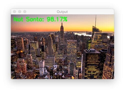
2020-06-03 Update: The image of the Manhattan skyline is no longer included in the “Downloads.” Updating this blog post to support TensorFlow 2+ led to a misclassification on this image. This figure remains in the post for legacy demonstration purposes, just realize that you won’t find it in the “Downloads.”
It looks like it’s too bright out for Santa to be flying through the sky and delivering presents in this part of the world yet (New York City) — he must still be in Europe at this time where night has fallen.
Speaking of the night and Christmas Eve, here is an image of a cold night sky:
$ python test_network.py --model santa_not_santa.model \
	--image examples/night_sky.png
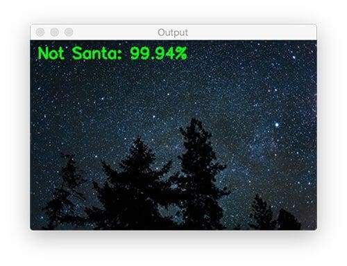
But it must be too early for St. Nicholas. He’s not in the above image either.
But don’t worry!
As I’ll show next week, we’ll be able to detect him sneaking down the chimney and delivering presents with a Raspberry Pi.
Limitations of our deep learning image classification model
There are a number of limitations to our image classifier.
The first one is that the 28×28 pixel images are quite small (the LeNet architecture was originally designed to recognize handwritten digits, not objects in photos).
For some example images (where Santa is already small), resizing the input image down to 28×28 pixels effectively reduces Santa down to a tiny red/white blob that is only 2-3 pixels in size.
In these types of situations it’s likely that our LeNet model is just predicting when there is a significant amount of red and white localized together in our input image (and likely green as well, as red, green, and white are Christmas colors).
State-of-the-art Convolutional Neural Networks normally accept images that are 200-300 pixels along their maximum dimension — these larger images would help us build a more robust Not Santa classifier. However, using larger resolution images would also require us to utilize a deeper network architecture, which in turn would mean that we need to gather additional training data and utilize a more computationally expensive training process.
This is certainly a possibility but is also outside the scope of this blog post.
Therefore, If you want to improve our Not Santa app I would suggest you:
- Gather additional training data (ideally, 5,000+ example “Santa” images).
- Utilize higher resolution images during training. I imagine 64×64 pixels would produce higher accuracy. 128×128 pixels would likely be ideal (although I have not tried this).
- Use a deeper network architecture during training.
- Read through my book, Deep Learning for Computer Vision with Python, where I discuss training Convolutional Neural Networks on your own custom datasets in more detail.
Despite these limitations, I was incredibly surprised with how well the Not Santa app performed (as I’ll discuss next week). I was expecting a decent number of false-positives but the network was surprisingly robust given how small it is.
What's next? We recommend PyImageSearch University.
86+ total classes • 115+ hours hours of on-demand code walkthrough videos • Last updated: April 2026
★★★★★ 4.84 (128 Ratings) • 16,000+ Students Enrolled
I strongly believe that if you had the right teacher you could master computer vision and deep learning.
Do you think learning computer vision and deep learning has to be time-consuming, overwhelming, and complicated? Or has to involve complex mathematics and equations? Or requires a degree in computer science?
That’s not the case.
All you need to master computer vision and deep learning is for someone to explain things to you in simple, intuitive terms. And that’s exactly what I do. My mission is to change education and how complex Artificial Intelligence topics are taught.
If you're serious about learning computer vision, your next stop should be PyImageSearch University, the most comprehensive computer vision, deep learning, and OpenCV course online today. Here you’ll learn how to successfully and confidently apply computer vision to your work, research, and projects. Join me in computer vision mastery.
Inside PyImageSearch University you'll find:
- ✓ 86+ courses on essential computer vision, deep learning, and OpenCV topics
- ✓ 86 Certificates of Completion
- ✓ 115+ hours hours of on-demand video
- ✓ Brand new courses released regularly, ensuring you can keep up with state-of-the-art techniques
- ✓ Pre-configured Jupyter Notebooks in Google Colab
- ✓ Run all code examples in your web browser — works on Windows, macOS, and Linux (no dev environment configuration required!)
- ✓ Access to centralized code repos for all 540+ tutorials on PyImageSearch
- ✓ Easy one-click downloads for code, datasets, pre-trained models, etc.
- ✓ Access on mobile, laptop, desktop, etc.
Summary
In today’s blog post you learned how to train the seminal LeNet architecture on a series of images containing “Santa” and “Not Santa”, with our end goal being to build an app similar to HBO’s Silicon Valley Not Hotdog application.
We were able to gather our “Santa” dataset (~460 images) by following our previous post on gathering deep learning images via Google Images.
The “Not Santa” dataset was created by sampling the UKBench dataset (where no images contain Santa).
We then evaluated our network on a series of testing images — in each case our Not Santa model correctly classified the input image.
In our next blog post, we’ll deploy our trained Convolutional Neural Network to the Raspberry Pi to finish building our Not Santa app.
What now?
Now that you’ve learned how to train your first Convolutional Neural Network, I’m willing to bet that you’re interested in:
- Mastering the fundamentals of machine learning and neural networks
- Studying deep learning in more detail
- Training your own Convolutional Neural Networks from scratch
If so, you’ll want to take a look at my new book, Deep Learning for Computer Vision with Python.
Inside the book you’ll find:
- Super-practical walkthroughs
- Hands-on tutorials (with lots of code)
- Detailed, thorough guides to help you replicate state-of-the-art results from seminal deep learning publications.
To learn more about my new book (and start your journey to deep learning mastery), just click here.
Otherwise, be sure to enter your email address in the form below to be notified when new deep learning posts are published here on PyImageSearch.

Download the Source Code and FREE 17-page Resource Guide
Enter your email address below to get a .zip of the code and a FREE 17-page Resource Guide on Computer Vision, OpenCV, and Deep Learning. Inside you'll find my hand-picked tutorials, books, courses, and libraries to help you master CV and DL!

