In this tutorial, we will be building a complete end-to-end application that can detect smiles in a video stream in real-time using deep learning along with traditional computer vision techniques.

To accomplish this task, we’ll be training the LetNet architecture on a dataset of images that contain faces of people who are smiling and not smiling. Once our network is trained, we’ll create a separate Python script — this one will detect faces in images via OpenCV’s built-in Haar cascade face detector, extract the face region of interest (ROI) from the image, and then pass the ROI through LeNet for smile detection.
To learn how to detect a smile with OpenCV, Keras, and TensorFlow, just keep reading.
Smile detection with OpenCV, Keras, and TensorFlow
When developing real-world applications for image classification, you’ll often have to mix traditional computer vision and image processing techniques with deep learning. I’ve done my best to ensure this tutorial stands on its own in terms of algorithms, techniques, and libraries you need to understand in order to be successful when studying and applying deep learning.
Configuring your development environment
To follow this guide, you need to have the OpenCV library installed on your system.
Luckily, OpenCV is pip-installable:
$ pip install opencv-contrib-python
If you need help configuring your development environment for OpenCV, I highly recommend that you read my pip install OpenCV guide — it will have you up and running in a matter of minutes.
Having problems configuring your development environment?
All that said, are you:
- Short on time?
- Learning on your employer’s administratively locked system?
- Wanting to skip the hassle of fighting with the command line, package managers, and virtual environments?
- Ready to run the code right now on your Windows, macOS, or Linux system?
Then join PyImageSearch University today!
Gain access to Jupyter Notebooks for this tutorial and other PyImageSearch guides that are pre-configured to run on Google Colab’s ecosystem right in your web browser! No installation required.
And best of all, these Jupyter Notebooks will run on Windows, macOS, and Linux!
The SMILES Dataset
The SMILES dataset consists of images of faces that are either smiling or not smiling (Hromada, 2010). In total, there are 13,165 grayscale images in the dataset, with each image having a size of 64×64 pixels.
As Figure 2 demonstrates, images in this dataset are tightly cropped around the face, which will make the training process easier as we’ll be able to learn the “smiling” or “not smiling” patterns directly from the input images.
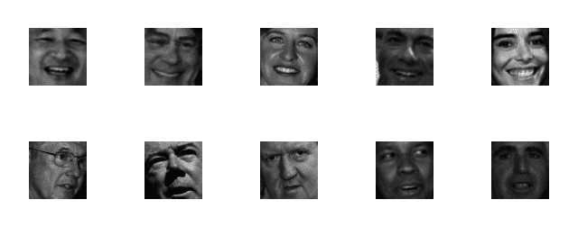
However, the close cropping poses a problem during testing — since our input images will not only contain a face but the background of the image as well, we first need to localize the face in the image and extract the face ROI before we can pass it through our network for detection. Luckily, using traditional computer vision methods such as Haar cascades, this is a much easier task than it sounds.
A second issue we need to handle in the SMILES dataset is class imbalance. While there are 13,165 images in the dataset, 9,475 of these examples are not smiling, while only 3,690 belong to the smiling class. Given that there are over 2.5x the number of “not smiling” images to “smiling” examples, we need to be careful when devising our training procedure.
Our network may naturally pick the “not smiling” label since (1) the distributions are uneven and (2) it has more examples of what a “not smiling” face looks like. Later, you will see how we can combat class imbalance by computing a “weight” for each class during training time.
Training the Smile CNN
The first step in building our smile detector is to train a CNN on the SMILES dataset to distinguish between a face that is smiling versus not smiling. To accomplish this task, let’s create a new file named train_model.py. From there, insert the following code:
# import the necessary packages
from sklearn.preprocessing import LabelEncoder
from sklearn.model_selection import train_test_split
from sklearn.metrics import classification_report
from tensorflow.keras.preprocessing.image import img_to_array
from tensorflow.keras.utils import to_categorical
from pyimagesearch.nn.conv import LeNet
from imutils import paths
import matplotlib.pyplot as plt
import numpy as np
import argparse
import imutils
import cv2
import os
Lines 2-14 import our required Python packages. We’ve used all of the packages before, but I want to call your attention to Line 7, where we import the LeNet (LeNet Tutorial) class — this is the architecture we’ll be using when creating our smile detector.
Next, let’s parse our command line arguments:
# construct the argument parse and parse the arguments
ap = argparse.ArgumentParser()
ap.add_argument("-d", "--dataset", required=True,
	help="path to input dataset of faces")
ap.add_argument("-m", "--model", required=True,
	help="path to output model")
args = vars(ap.parse_args())

# initialize the list of data and labels
data = []
labels = []
Our script will require two command line arguments, each of which I’ve detailed below:
--dataset: The path to the SMILES directory residing on disk.--model: The path to where the serialized LeNet weights will be saved after training.
We are now ready to load the SMILES dataset from disk and store it in memory:
# loop over the input images
for imagePath in sorted(list(paths.list_images(args["dataset"]))):
	# load the image, pre-process it, and store it in the data list
	image = cv2.imread(imagePath)
	image = cv2.cvtColor(image, cv2.COLOR_BGR2GRAY)
	image = imutils.resize(image, width=28)
	image = img_to_array(image)
	data.append(image)

	# extract the class label from the image path and update the
	# labels list
	label = imagePath.split(os.path.sep)[-3]
	label = "smiling" if label == "positives" else "not_smiling"
	labels.append(label)
On Line 29, we loop over all images in the --dataset input directory. For each of these images, we:
- Load it from disk (Line 31).
- Convert it to grayscale (Line 32).
- Resize it to have a fixed input size of
28×28pixels (Line 33). - Convert the image to an array compatible with Keras and its channel ordering (Line 34).
- Add the
imageto thedatalist that LeNet will be trained on.
Lines 39-41 handle extracting the class label from the imagePath and updating the labels list. The SMILES dataset stores smiling faces in the SMILES/positives/positives7 subdirectory, while not smiling faces live in the SMILES/negatives/negatives7 subdirectory.
Therefore, given the path to an image:
SMILEs/positives/positives7/10007.jpg
We can extract the class label by splitting on the image path separator and grabbing the third-to-last subdirectory: positives. In fact, this is exactly what Line 39 accomplishes.
Now that our data and labels are constructed, we can scale the raw pixel intensities to the range [0, 1] and then apply one-hot encoding to the labels:
# scale the raw pixel intensities to the range [0, 1]
data = np.array(data, dtype="float") / 255.0
labels = np.array(labels)

# convert the labels from integers to vectors
le = LabelEncoder().fit(labels)
labels = to_categorical(le.transform(labels), 2)
Our next code block handles our data imbalance issue by computing the class weights:
# calculate the total number of training images in each class and
# initialize a dictionary to store the class weights
classTotals = labels.sum(axis=0)
classWeight = dict()

# loop over all classes and calculate the class weight
for i in range(0, len(classTotals)):
	classWeight[i] = classTotals.max() / classTotals[i]
Line 53 computes the total number of examples per class. In this case, classTotals will be an array: [9475, 3690] for “not smiling” and “smiling,” respectively.
We then scale these totals on Lines 57 and 58 to obtain the classWeight used to handle the class imbalance, yielding the array: [1, 2.56]. This weighting implies that our network will treat every instance of “smiling” as 2.56 instances of “not smiling” and helps combat the class imbalance issue by amplifying the per-instance loss by a larger weight when seeing “smiling” examples.
Now that we’ve computed our class weights, we can move on to partitioning our data into training and testing splits, using 80% of the data for training and 20% for testing:
# partition the data into training and testing splits using 80% of
# the data for training and the remaining 20% for testing
(trainX, testX, trainY, testY) = train_test_split(data,
	labels, test_size=0.20, stratify=labels, random_state=42)
Finally, we are ready to train LeNet:
# initialize the model
print("[INFO] compiling model...")
model = LeNet.build(width=28, height=28, depth=1, classes=2)
model.compile(loss="binary_crossentropy", optimizer="adam",
	metrics=["accuracy"])

# train the network
print("[INFO] training network...")
H = model.fit(trainX, trainY, validation_data=(testX, testY),
	class_weight=classWeight, batch_size=64, epochs=15, verbose=1)
Line 67 initializes the LeNet architecture that will accept 28×28 single channel images. Given that there are only two classes (smiling versus not smiling), we set classes=2.
We’ll also be using binary_crossentropy rather than categorical_crossentropy as our loss function. Again, categorical cross-entropy is only used when the number of classes is more than two.
Up until this point, we’ve been using the SGD optimizer to train our network. Here, we’ll be using Adam (Kingma and Ba, 2014) (Line 68).
Again, the optimizer and associated parameters are often considered hyperparameters that you need to tune when training your network. When I put this example together, I found that Adam performed substantially better than SGD.
Lines 73 and 74 train LeNet for a total of 15 epochs using our supplied classWeight to combat class imbalance.
Once our network is trained, we can evaluate it and serialize the weights to disk:
# evaluate the network
print("[INFO] evaluating network...")
predictions = model.predict(testX, batch_size=64)
print(classification_report(testY.argmax(axis=1),
	predictions.argmax(axis=1), target_names=le.classes_))

# save the model to disk
print("[INFO] serializing network...")
model.save(args["model"])
We’ll also construct a learning curve for our network so we can visualize performance:
# plot the training + testing loss and accuracy
plt.style.use("ggplot")
plt.figure()
plt.plot(np.arange(0, 15), H.history["loss"], label="train_loss")
plt.plot(np.arange(0, 15), H.history["val_loss"], label="val_loss")
plt.plot(np.arange(0, 15), H.history["accuracy"], label="acc")
plt.plot(np.arange(0, 15), H.history["val_accuracy"], label="val_acc")
plt.title("Training Loss and Accuracy")
plt.xlabel("Epoch #")
plt.ylabel("Loss/Accuracy")
plt.legend()
plt.show()
To train our smile detector, execute the following command:
$ python train_model.py --dataset ../datasets/SMILEsmileD \
	--model output/lenet.hdf5
[INFO] compiling model...
[INFO] training network...
Train on 10532 samples, validate on 2633 samples
Epoch 1/15
8s - loss: 0.3970 - acc: 0.8161 - val_loss: 0.2771 - val_acc: 0.8872
Epoch 2/15
8s - loss: 0.2572 - acc: 0.8919 - val_loss: 0.2620 - val_acc: 0.8899
Epoch 3/15
7s - loss: 0.2322 - acc: 0.9079 - val_loss: 0.2433 - val_acc: 0.9062
...
Epoch 15/15
8s - loss: 0.0791 - acc: 0.9716 - val_loss: 0.2148 - val_acc: 0.9351
[INFO] evaluating network...
             precision    recall  f1-score   support

not_smiling       0.95      0.97      0.96      1890
    smiling       0.91      0.86      0.88       743

avg / total       0.93      0.94      0.93      2633

[INFO] serializing network...
After 15 epochs, we can see that our network is obtaining 93% classification accuracy. Figure 3 plots our learning curve:
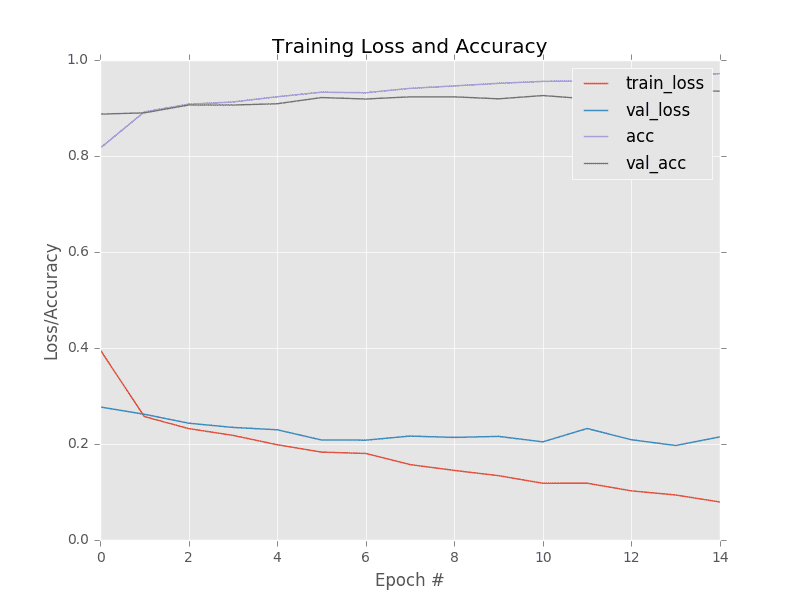
Past epoch six our validation loss starts to stagnate — further training past epoch 15 would result in overfitting. If desired, we would improve the accuracy of our smile detector by using more training data, either by:
- Gathering additional training data.
- Applying data augmentation to randomly translate, rotate, and shift our existing training set.
Running the Smile CNN in Real-time
Now that we’ve trained our model, the next step is to build the Python script to access our webcam/video file and apply smile detection to each frame. To accomplish this step, open a new file, name it detect_smile.py, and we’ll get to work.
# import the necessary packages
from tensorflow.keras.preprocessing.image import img_to_array
from tensorflow.keras.models import load_model
import numpy as np
import argparse
import imutils
import cv2
Lines 2-7 import our required Python packages. The img_to_array function will be used to convert each individual frame from our video stream to a properly channel ordered array. The load_model function will be used to load the weights of our trained LeNet model from disk.
The detect_smile.py script requires two command line arguments followed by a third optional one:
# construct the argument parse and parse the arguments
ap = argparse.ArgumentParser()
ap.add_argument("-c", "--cascade", required=True,
	help="path to where the face cascade resides")
ap.add_argument("-m", "--model", required=True,
	help="path to pre-trained smile detector CNN")
ap.add_argument("-v", "--video",
	help="path to the (optional) video file")
args = vars(ap.parse_args())
The first argument, --cascade is the path to a Haar cascade used to detect faces in images. First published in 2001, Paul Viola and Michael Jones detail the Haar cascade in their work, Rapid Object Detection using a Boosted Cascade of Simple Features. This publication has become one of the most cited papers in the computer vision literature.
The Haar cascade algorithm is capable of detecting objects in images, regardless of their location and scale. Perhaps most intriguing (and relevant to our application), the detector can run in real-time on modern hardware. In fact, the motivation behind Viola and Jones’ work was to create a face detector.
The second common line argument, --model, specifies the path to our serialized LeNet weights on disk. Our script will default to reading frames from a built-in/USB webcam; however, if we instead want to read frames from a file, we can specify the file via the optional --video switch.
Before we can detect smiles, we first need to perform some initializations:
# load the face detector cascade and smile detector CNN
detector = cv2.CascadeClassifier(args["cascade"])
model = load_model(args["model"])

# if a video path was not supplied, grab the reference to the webcam
if not args.get("video", False):
	camera = cv2.VideoCapture(0)

# otherwise, load the video
else:
	camera = cv2.VideoCapture(args["video"])
Lines 20 and 21 load the Haar cascade face detector and the pre-trained LeNet model, respectively. If a video path was not supplied, we grab a pointer to our webcam (Lines 24 and 25). Otherwise, we open a pointer to the video file on disk (Lines 28 and 29).
We have now reached the main processing pipeline of our application:
# keep looping
while True:
	# grab the current frame
	(grabbed, frame) = camera.read()

	# if we are viewing a video and we did not grab a frame, then we
	# have reached the end of the video
	if args.get("video") and not grabbed:
		break

	# resize the frame, convert it to grayscale, and then clone the
	# original frame so we can draw on it later in the program
	frame = imutils.resize(frame, width=300)
	gray = cv2.cvtColor(frame, cv2.COLOR_BGR2GRAY)
	frameClone = frame.copy()
Line 32 starts a loop that will continue until (1) we stop the script or (2) we reach the end of the video file (provided a --video path was applied).
Line 34 grabs the next frame from the video stream. If the frame could not be grabbed, then we have reached the end of the video file. Otherwise, we pre-process the frame for face detection by resizing it to have a width of 300 pixels (Line 43) and converting it to grayscale (Line 44).
The .detectMultiScale method handles detecting the bounding box (x, y)-coordinates of faces in the frame:
	# detect faces in the input frame, then clone the frame so that
	# we can draw on it
	rects = detector.detectMultiScale(gray, scaleFactor=1.1,
		minNeighbors=5, minSize=(30, 30),
		flags=cv2.CASCADE_SCALE_IMAGE)
Here, we pass in our grayscale image and indicate that for a given region to be considered a face it must have a minimum width of 30×30 pixels. The minNeighbors attribute helps prune false positives while the scaleFactor controls the number of image pyramid (http://pyimg.co/rtped) levels generated.
Again, a detailed review of Haar cascades for object detection is outside the scope of this tutorial.
The .detectMultiScale method returns a list of 4-tuples that make up the rectangle that bounds the face in the frame. The first two values in this list are the starting (x, y)-coordinates. The second two values in the rects list are the width and height of the bounding box, respectively.
We loop over each set of bounding boxes below:
	# loop over the face bounding boxes
	for (fX, fY, fW, fH) in rects:
		# extract the ROI of the face from the grayscale image,
		# resize it to a fixed 28x28 pixels, and then prepare the
		# ROI for classification via the CNN
		roi = gray[fY:fY + fH, fX:fX + fW]
		roi = cv2.resize(roi, (28, 28))
		roi = roi.astype("float") / 255.0
		roi = img_to_array(roi)
		roi = np.expand_dims(roi, axis=0)
For each of the bounding boxes, we use NumPy array slicing to extract the face ROI (Line 58). Once we have the ROI, we preprocess it and prepare it for classification via LeNet by resizing it, scaling it, converting it to a Keras-compatible array, and padding the image with an extra dimension (Lines 59-62).
Once the roi is preprocessed, it can be passed through LeNet for classification:
		# determine the probabilities of both "smiling" and "not
		# smiling", then set the label accordingly
		(notSmiling, smiling) = model.predict(roi)[0]
		label = "Smiling" if smiling > notSmiling else "Not Smiling"
A call to .predict on Line 66 returns the probabilities of “not smiling” and “smiling,” respectively. Line 67 sets the label depending on which probability is larger.
Once we have the label, we can draw it, along with the corresponding bounding box on the frame:
		# display the label and bounding box rectangle on the output
		# frame
		cv2.putText(frameClone, label, (fX, fY - 10),
			cv2.FONT_HERSHEY_SIMPLEX, 0.45, (0, 0, 255), 2)
		cv2.rectangle(frameClone, (fX, fY), (fX + fW, fY + fH),
			(0, 0, 255), 2)
Our final code block handles displaying the output frame on our screen:
	# show our detected faces along with smiling/not smiling labels
	cv2.imshow("Face", frameClone)

	# if the 'q' key is pressed, stop the loop
	if cv2.waitKey(1) & 0xFF == ord("q"):
		break

# cleanup the camera and close any open windows
camera.release()
cv2.destroyAllWindows()
If the q key is pressed, we exit the script.
To run detect_smile.py using your webcam, execute the following command:
$ python detect_smile.py --cascade haarcascade_frontalface_default.xml \
	--model output/lenet.hdf5
If you instead want to use a video file, you would update your command to use the --video switch:
$ python detect_smile.py --cascade haarcascade_frontalface_default.xml \
	--model output/lenet.hdf5 --video path/to/your/video.mov
I have included the results of the smile detection script in Figure 4:
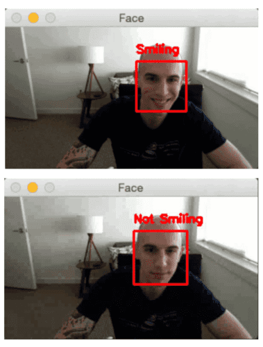
Notice how LeNet is correctly predicting “smiling” or “not smiling” based on my facial expression.
What's next? We recommend PyImageSearch University.
86+ total classes • 115+ hours hours of on-demand code walkthrough videos • Last updated: April 2026
★★★★★ 4.84 (128 Ratings) • 16,000+ Students Enrolled
I strongly believe that if you had the right teacher you could master computer vision and deep learning.
Do you think learning computer vision and deep learning has to be time-consuming, overwhelming, and complicated? Or has to involve complex mathematics and equations? Or requires a degree in computer science?
That’s not the case.
All you need to master computer vision and deep learning is for someone to explain things to you in simple, intuitive terms. And that’s exactly what I do. My mission is to change education and how complex Artificial Intelligence topics are taught.
If you're serious about learning computer vision, your next stop should be PyImageSearch University, the most comprehensive computer vision, deep learning, and OpenCV course online today. Here you’ll learn how to successfully and confidently apply computer vision to your work, research, and projects. Join me in computer vision mastery.
Inside PyImageSearch University you'll find:
- ✓ 86+ courses on essential computer vision, deep learning, and OpenCV topics
- ✓ 86 Certificates of Completion
- ✓ 115+ hours hours of on-demand video
- ✓ Brand new courses released regularly, ensuring you can keep up with state-of-the-art techniques
- ✓ Pre-configured Jupyter Notebooks in Google Colab
- ✓ Run all code examples in your web browser — works on Windows, macOS, and Linux (no dev environment configuration required!)
- ✓ Access to centralized code repos for all 540+ tutorials on PyImageSearch
- ✓ Easy one-click downloads for code, datasets, pre-trained models, etc.
- ✓ Access on mobile, laptop, desktop, etc.
Summary
In this tutorial, we learned how to build an end-to-end computer vision and deep learning application to perform smile detection. To do so, we first trained the LeNet architecture on the SMILES dataset. Due to class imbalances in the SMILES dataset, we discovered how to compute class weights used to help mitigate the problem.
Once trained, we evaluated LeNet on our testing set and found the network obtained a respectable 93% classification accuracy. Higher classification accuracy can be obtained by gathering more training data or applying data augmentation to existing training data.
We then created a Python script to read frames from a webcam/video file, detect faces, and then apply our pre-trained network. To detect faces, we used OpenCV’s Haar cascades. Once a face was detected it was extracted from the frame and then passed through LeNet to determine if the person was smiling or not smiling. As a whole, our smile detection system can easily run in real-time on the CPU using modern hardware.
To download the source code to this post (and be notified when future tutorials are published here on PyImageSearch), simply enter your email address in the form below!

Download the Source Code and FREE 17-page Resource Guide
Enter your email address below to get a .zip of the code and a FREE 17-page Resource Guide on Computer Vision, OpenCV, and Deep Learning. Inside you'll find my hand-picked tutorials, books, courses, and libraries to help you master CV and DL!


Comment section
Hey, Adrian Rosebrock here, author and creator of PyImageSearch. While I love hearing from readers, a couple years ago I made the tough decision to no longer offer 1:1 help over blog post comments.
At the time I was receiving 200+ emails per day and another 100+ blog post comments. I simply did not have the time to moderate and respond to them all, and the sheer volume of requests was taking a toll on me.
Instead, my goal is to do the most good for the computer vision, deep learning, and OpenCV community at large by focusing my time on authoring high-quality blog posts, tutorials, and books/courses.
If you need help learning computer vision and deep learning, I suggest you refer to my full catalog of books and courses — they have helped tens of thousands of developers, students, and researchers just like yourself learn Computer Vision, Deep Learning, and OpenCV.
Click here to browse my full catalog.