Last updated on July 4, 2021.
In this tutorial, you will learn how the Keras .fit and .fit_generator functions work, including the differences between them. To help you gain hands-on experience, I’ve included a full example showing you how to implement a Keras data generator from scratch.
A large dataset is crucial when using Keras’ fit and fit_generator functions. It allows us to understand the difference between the two and observe how they handle data of large volumes.
Roboflow has free tools for each stage of the computer vision pipeline that will streamline your workflows and supercharge your productivity.
Sign up or Log in to your Roboflow account to access state of the art dataset libaries and revolutionize your computer vision pipeline.
You can start by choosing your own datasets or using our PyimageSearch’s assorted library of useful datasets.
Bring data in any of 40+ formats to Roboflow, train using any state-of-the-art model architectures, deploy across multiple platforms (API, NVIDIA, browser, iOS, etc), and connect to applications or 3rd party tools.
Today’s blog post is inspired by PyImageSearch reader, Shey.
Shey asks:
Hi Adrian, thanks for your tutorials. I’ve been methodically going through every one. They’ve really helped me learn deep learning.
I have a question about the Keras “.fit_generator” function.
I’ve noticed you use it quite a bit in your blog posts but I’m not really sure how the function is different than Keras’ standard “.fit” function.
How is it different? How do I know when to use each? And how to I create a data generator for the “.fit_generator” function?
Shey asks a great question.
The Keras deep learning library includes three separate functions that can be used to train your own models:
.fit.fit_generator.train_on_batch
If you’re new to Keras and deep learning you may feel a bit overwhelmed trying to determine which function you’re supposed to use — this confusion is only compounded if you need to work with your own custom data.
To help lift the cloud of confusion regarding the Keras fit and fit_generator functions, I’m going to spend this tutorial discussing:
- The differences between Keras’
.fit,.fit_generator, and.train_on_batchfunctions - When to use each when training your own deep learning models
- How to implement your own Keras data generator and utilize it when training a model using
.fit_generator - How to use the
.predict_generatorfunction when evaluating your network after training
To learn more about Keras’ .fit and .fit_generator functions, including how to train a deep learning model on your own custom dataset, just keep reading!
- Update July 2021: For TensorFlow 2.2+ users, just use the
.fitmethod for your projects. The.fit_generatormethod will be deprecated in future releases of TensorFlow as the.fitmethod can automatically detect if the input data is an array or a generator.
How to use Keras fit and fit_generator (a hands-on tutorial)
2020-05-13 Update: This blog post is now TensorFlow 2+ compatible! TensorFlow is in the process of deprecating the .fit_generator method which supported data augmentation. If you are using tensorflow==2.2.0 or tensorflow-gpu==2.2.0 (or higher), then you must use the .fit method (which now supports data augmentation). Please keep this in mind while reading this legacy tutorial. Of course the concept of data augmentation stays the same. Please note that the code in the tutorial is updated for TensorFlow 2.2+ compatibility, however you may still see in-text references for the legacy .fit_generator method.
In the first part of today’s tutorial we’ll discuss the differences between Keras’ .fit, .fit_generator, and .train_on_batch functions.
From there I’ll show you an example of a “non-standard” image dataset which doesn’t contain any actual PNG, JPEG, etc. images at all! Instead, the entire image dataset is represented by two CSV files, one for training and the second for evaluation.
Our goal will be to implement a Keras generator capable of training a network on this CSV image data (don’t worry, I’ll show you how to implement such a generator function from scratch).
Finally, we’ll train and evaluate our network.
When to use Keras’ fit, fit_generator, and train_on_batch functions?
Keras provides three functions that can be used to train your own deep learning models:
.fit.fit_generator.train_on_batch
All three of these functions can essentially accomplish the same task — but how they go about doing it is very different.
Let’s explore each of these functions one-by-one, looking at an example function call, and then discussing how they are different from each other.
The Keras .fit function
Let’s start with a call to .fit :
model.fit(trainX, trainY, batch_size=32, epochs=50)
Here you can see that we are supplying our training data (trainX ) and training labels (trainY ).
We then instruct Keras to allow our model to train for 50 epochs with a batch size of 32 .
The call to .fit is making two primary assumptions here:
- Our entire training set can fit into RAM
- There is no data augmentation going on (i.e., there is no need for Keras generators)
Instead, our network will be trained on the raw data.
The raw data itself will fit into memory — we have no need to move old batches of data out of RAM and move new batches of data into RAM.
Furthermore, we will not be manipulating the training data on the fly using data augmentation.
The Keras fit_generator function
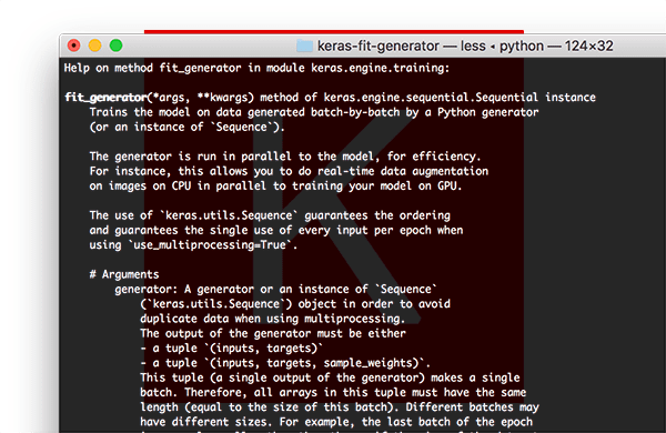
.fit_generator function allows for data augmentation and data generators.For small, simplistic datasets it’s perfectly acceptable to use Keras’ .fit function.
These datasets are often not very challenging and do not require any data augmentation.
However, real-world datasets are rarely that simple:
- Real-world datasets are often too large to fit into memory.
- They also tend to be challenging, requiring us to perform data augmentation to avoid overfitting and increase the ability of our model to generalize.
In those situations we need to utilize Keras’ .fit_generator function:
# initialize the number of epochs and batch size
EPOCHS = 100
BS = 32

# construct the training image generator for data augmentation
aug = ImageDataGenerator(rotation_range=20, zoom_range=0.15,
	width_shift_range=0.2, height_shift_range=0.2, shear_range=0.15,
	horizontal_flip=True, fill_mode="nearest")

# train the network
H = model.fit_generator(aug.flow(trainX, trainY, batch_size=BS),
	validation_data=(testX, testY), steps_per_epoch=len(trainX) // BS,
	epochs=EPOCHS)
2020-05-13 Update: With TensorFlow 2.2+ we now use .fit instead of .fit_generator which works the exact same way under the hood to accommodate data augmentation if the first argument provided is a Python generator object.
Here we start by first initializing the number of epochs we are going to train our network for along with the batch size.
We then initialize aug , a Keras ImageDataGenerator object that is used to apply data augmentation, randomly translating, rotating, resizing, etc. images on the fly.
Performing data augmentation is a form of regularization, enabling our model to generalize better.
However, applying data augmentation implies that our training data is no longer “static” — the data is constantly changing.
Each new batch of data is randomly adjusted according to the parameters supplied to ImageDataGenerator .
Thus, we now need to utilize Keras’ .fit_generator function to train our model.
As the name suggests, the .fit_generator function assumes there is an underlying function that is generating the data for it.
The function itself is a Python generator.
Internally, Keras is using the following process when training a model with .fit_generator :
- Keras calls the generator function supplied to
.fit_generator(in this case,aug.flow). - The generator function yields a batch of size
BSto the.fit_generatorfunction. - The
.fit_generatorfunction accepts the batch of data, performs backpropagation, and updates the weights in our model. - This process is repeated until we have reached the desired number of epochs.
You’ll notice we now need to supply a steps_per_epoch parameter when calling .fit_generator (the .fit method had no such parameter).
Why do we need steps_per_epoch ?
Keep in mind that a Keras data generator is meant to loop infinitely — it should never return or exit.
Since the function is intended to loop infinitely, Keras has no ability to determine when one epoch starts and a new epoch begins.
Therefore, we compute the steps_per_epoch value as the total number of training data points divided by the batch size. Once Keras hits this step count it knows that it’s a new epoch.
The Keras train_on_batch function
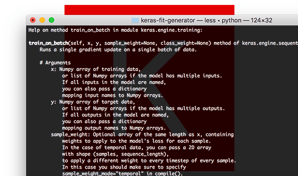
.train_on_batch function in Keras offers expert-level control over training Keras models.For deep learning practitioners looking for the finest-grained control over training your Keras models, you may wish to use the .train_on_batch function:
model.train_on_batch(batchX, batchY)
The train_on_batch function accepts a single batch of data, performs backpropagation, and then updates the model parameters.
The batch of data can be of arbitrary size (i.e., it does not require an explicit batch size to be provided).
The data itself can be generated however you like as well. This data could be raw images on disk or data that has been modified or augmented in some manner.
You’ll typically use the .train_on_batch function when you have very explicit reasons for wanting to maintain your own training data iterator, such as the data iteration process being extremely complex and requiring custom code.
If you find yourself asking if you need the .train_on_batch function then in all likelihood you probably don’t.
In 99% of the situations you will not need such fine-grained control over training your deep learning models. Instead, a custom Keras .fit_generator function is likely all you need it.
That said, it’s good to know that the function exists if you ever need it.
I typically only recommend using the .train_on_batch function if you are an advanced deep learning practitioner/engineer, and you know exactly what you’re doing and why.
An image dataset…as a CSV file?
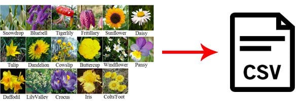
The dataset we will be using here today is the Flowers-17 dataset, a collection of 17 different flower species with 80 images per class.
Our goal will be to train a Keras Convolutional Neural Network to correctly classify each species of flowers.
However, there’s a bit of a twist to this project:
- Instead of working with the raw image files residing on disk…
- …I’ve serialized the entire image dataset to two CSV files (one for training, and one for evaluation).
To construct each CSV file I:
- Looped over all images in our input dataset
- Resized them to 64×64 pixels
- Flattened the 64x64x3=12,288 RGB pixel intensities into a single list
- Wrote 12,288 pixel values + class label to the CSV file (one per line)
Our goal is to now write a custom Keras generator to parse the CSV file and yield batches of images and labels to the .fit_generator function.
Wait, why bother with a CSV file if you already have the images?
Today’s tutorial is meant to be an example of how to implement your own Keras generator for the .fit_generator function.
In the real-world datasets are not nicely curated for you:
- You may have unstructured directories of images.
- You could be working with both images and text.
- Your images could be serialized in a particular format, whether that’s a CSV file, a Caffe or TensorFlow record file, etc.
In these situations, you will need to know how to write your own Keras generator functions.
Keep in mind that it’s not the particular data format that’s important here — it’s the actual process of writing your own Keras generator that you need to learn (and that’s exactly what’s covered in the rest of the tutorial).
Project structure
Let’s inspect the project tree for today’s example:
$ tree --dirsfirst
.
├── pyimagesearch
│   ├── __init__.py
│   └── minivggnet.py
├── flowers17_testing.csv
├── flowers17_training.csv
├── plot.png
└── train.py

1 directory, 6 files
Today we’ll be using the MiniVGGNet CNN. We won’t be covering the implementation here today as I’ll assume you already know how to implement a CNN. If not, no worries — just refer to my Keras tutorial.
Our serialized image dataset is contained within flowers17_training.csv and flowers17_testing.csv (included in the “Downloads” associated with today’s post).
We’ll be reviewing train.py , our training script, in the next two sections.
Implementing a custom Keras fit_generator function
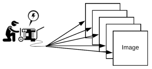
ImageDataGenerator from Keras coupled with our custom csv_image_generator. The generator will burn the CSV fuel to create batches of images for training.Let’s go ahead and get started.
I’ll be assuming you have the following libraries installed on your system:
- NumPy
- TensorFlow + Keras
- Scikit-learn
- Matplotlib
Each of these packages can be installed via pip in your virtual environment. If you have virtualenvwrapper installed you can create an environment with mkvirtualenv and activate your environment with the workon command. From there you can use pip to set up your environment:
$ mkvirtualenv cv -p python3
$ workon cv
$ pip install numpy
$ pip install tensorflow # or tensorflow-gpu
$ pip install keras
$ pip install scikit-learn
$ pip install matplotlib
Once your virtual environment is set up, you can proceed with writing the training script. Make sure you use the “Downloads” section of today’s post grab the source code and Flowers-17 CSV image dataset.
Open up the train.py file and insert the following code:
# set the matplotlib backend so figures can be saved in the background
import matplotlib
matplotlib.use("Agg")

# import the necessary packages
from tensorflow.keras.preprocessing.image import ImageDataGenerator
from tensorflow.keras.optimizers import SGD
from sklearn.preprocessing import LabelBinarizer
from sklearn.metrics import classification_report
from pyimagesearch.minivggnet import MiniVGGNet
import matplotlib.pyplot as plt
import numpy as np
Lines 2-12 import our required packages and modules. Since we’ll be saving our training plot to disk, Line 3 sets matplotlib ‘s backend appropriately.
Notable imports include ImageDataGenerator , which contains the data augmentation and image generator functionality, along with MiniVGGNet , our CNN that we will be training.
Let’s define the csv_image_generator function:
def csv_image_generator(inputPath, bs, lb, mode="train", aug=None):
	# open the CSV file for reading
	f = open(inputPath, "r")
On Line 14 we’ve defined the csv_image_generator . This function is responsible for reading our CSV data file and loading images into memory. It yields batches of data to our Keras .fit_generator function.
As such, the function accepts the following parameters:
inputPath: the path to the CSV dataset file.bs: The batch size. We’ll be using 32.lb: A label binarizer object which contains our class labels.mode: (default is"train") If and only if themode=="eval", then a special accommodation is made to not apply data augmentation via theaugobject (if one is supplied).aug: (default isNone) If an augmentation object is specified, then we’ll apply it before we yield our images and labels.
On Line 16 we’ll go ahead and open the CSV data file for reading.
Let’s begin looping over the lines of data:
	# loop indefinitely
	while True:
		# initialize our batches of images and labels
		images = []
		labels = []
Each line of data in the CSV file contains an image serialized as a text string. Again, I generated the text strings from the Flowers-17 dataset. Additionally, I know this isn’t the most efficient way to store an image, but it is great for the purposes of this example.
Our Keras generator must loop indefinitely as is defined on Line 19. The .fit_generator function will be calling our csv_image_generator function each time it needs a new batch of data.
And furthermore, Keras maintains a cache/queue of data, ensuring the model we are training always has data to train on. Keras constantly keeps this queue full so even if you have reached the total number of epochs to train for, keep in mind that Keras is still feeding the data generator, keeping data in the queue.
Always make sure your function returns data, otherwise, Keras will error out saying it could not obtain more training data from your generator.
At each iteration of the loop, we’ll reinitialize our images and labels to empty lists (Lines 21 and 22).
From there, we’ll begin appending images and labels to these lists until we’ve reached our batch size:
		# keep looping until we reach our batch size
		while len(images) < bs:
			# attempt to read the next line of the CSV file
			line = f.readline()

			# check to see if the line is empty, indicating we have
			# reached the end of the file
			if line == "":
				# reset the file pointer to the beginning of the file
				# and re-read the line
				f.seek(0)
				line = f.readline()

				# if we are evaluating we should now break from our
				# loop to ensure we don't continue to fill up the
				# batch from samples at the beginning of the file
				if mode == "eval":
					break

			# extract the label and construct the image
			line = line.strip().split(",")
			label = line[0]
			image = np.array([int(x) for x in line[1:]], dtype="float32")
			image = image.reshape((64, 64, 3))

			# update our corresponding batches lists
			images.append(image)
			labels.append(label)
Let’s walk through this loop:
- First, we read a
linefrom our text file object,f(Line 27). - If
lineis empty:- …we reset our file pointer and try to read a
line(Lines 34 and 35). - And if we’re in evaluation
mode, we go ahead andbreakfrom the loop (Lines 40 and 41).
- …we reset our file pointer and try to read a
- At this point, we’ll parse our
imageandlabelfrom the CSV file (Lines 44-46). - We go ahead and call
.reshapeto reshape our 1D array into our image which is 64×64 pixels with 3 color channels (Line 47). - Finally, we append the
imageandlabelto their respective lists, repeating this process until our batch of images is full (Lines 50 and 51).
Note: The key to making evaluation work here is that we supply the number of steps to model.predict_generator , ensuring that each image in the testing set is predicted only once. I’ll be covering how to do this process later in the tutorial.
With our batch of images and corresponding labels ready, we can now take two steps before yielding our batch:
		# one-hot encode the labels
		labels = lb.transform(np.array(labels))

		# if the data augmentation object is not None, apply it
		if aug is not None:
			(images, labels) = next(aug.flow(np.array(images),
				labels, batch_size=bs))

		# yield the batch to the calling function
		yield (np.array(images), labels)
Our final steps include:
- One-hot encoding
labels(Line 54) - Applying data augmentation if necessary (Lines 57-59)
Finally, our generator “yields” our array of images and our list of labels to the calling function on request (Line 62). If you aren’t familiar with the yield keyword, it is used for Python Generator functions as a convenient shortcut in place of building an iterator class with less memory consumption. You can read more about Python Generators here.
Let’s initialize our training parameters:
# initialize the paths to our training and testing CSV files
TRAIN_CSV = "flowers17_training.csv"
TEST_CSV = "flowers17_testing.csv"

# initialize the number of epochs to train for and batch size
NUM_EPOCHS = 75
BS = 32

# initialize the total number of training and testing image
NUM_TRAIN_IMAGES = 0
NUM_TEST_IMAGES = 0
A number of initializations are hardcoded in this example training script:
- Our training and testing CSV filepaths (Lines 65 and 66).
- The number of epochs and batch size for training (Lines 69 and 70).
- Two variables which will hold the number of training and testing images (Lines 73 and 74).
Let’s take a look at the next block of code:
# open the training CSV file, then initialize the unique set of class
# labels in the dataset along with the testing labels
f = open(TRAIN_CSV, "r")
labels = set()
testLabels = []

# loop over all rows of the CSV file
for line in f:
	# extract the class label, update the labels list, and increment
	# the total number of training images
	label = line.strip().split(",")[0]
	labels.add(label)
	NUM_TRAIN_IMAGES += 1

# close the training CSV file and open the testing CSV file
f.close()
f = open(TEST_CSV, "r")

# loop over the lines in the testing file
for line in f:
	# extract the class label, update the test labels list, and
	# increment the total number of testing images
	label = line.strip().split(",")[0]
	testLabels.append(label)
	NUM_TEST_IMAGES += 1

# close the testing CSV file
f.close()
This block of code is long, but it has three purposes:
- Extract all labels from our training dataset so that we can subsequently determine unique labels. Notice that
labelsis asetwhich only allows unique entries. - Assemble a list of
testLabels. - Count the
NUM_TRAIN_IMAGESandNUM_TEST_IMAGES.
Let’s build our LabelBinarizer object and construct the data augmentation object:
# create the label binarizer for one-hot encoding labels, then encode
# the testing labels
lb = LabelBinarizer()
lb.fit(list(labels))
testLabels = lb.transform(testLabels)

# construct the training image generator for data augmentation
aug = ImageDataGenerator(rotation_range=20, zoom_range=0.15,
	width_shift_range=0.2, height_shift_range=0.2, shear_range=0.15,
	horizontal_flip=True, fill_mode="nearest")
Using the unique labels, we’ll .fit our LabelBinarizer object (Lines 107 and 108).
We’ll also go ahead and transform our testLabels into binary one-hot encoded testLabels (Line 109).
From there, we’ll construct aug , an ImageDataGenerator (Lines 112-114). Our image data augmentation object will randomly rotate, flip, shear, etc. our training images.
Now let’s initialize our training and testing image generators:
# initialize both the training and testing image generators
trainGen = csv_image_generator(TRAIN_CSV, BS, lb,
	mode="train", aug=aug)
testGen = csv_image_generator(TEST_CSV, BS, lb,
	mode="train", aug=None)
Our trainGen and testGen generator objects generate image data from their respective CSV files using the csv_image_generator (Lines 117-120).
Notice the subtle similarities and differences:
- We’re using
mode="train"for both generators - Only
trainGenwill perform data augmentation
Let’s initialize + compile our MiniVGGNet model with Keras and begin training:
# initialize our Keras model and compile it
model = MiniVGGNet.build(64, 64, 3, len(lb.classes_))
opt = SGD(lr=1e-2, momentum=0.9, decay=1e-2 / NUM_EPOCHS)
model.compile(loss="categorical_crossentropy", optimizer=opt,
	metrics=["accuracy"])

# train the network
print("[INFO] training w/ generator...")
H = model.fit(
	x=trainGen,
	steps_per_epoch=NUM_TRAIN_IMAGES // BS,
	validation_data=testGen,
	validation_steps=NUM_TEST_IMAGES // BS,
	epochs=NUM_EPOCHS)
2020-05-13 Update: This blog post is now TensorFlow 2+ compatible! We no-longer use the .fit_generator function; instead, we use the .fit method.
Lines 123-126 compile our model. We’re using a Stochastic Gradient Descent optimizer with a hardcoded initial learning rate of 1e-2 . Learning rate decay is applied at each epoch. Categorical crossentropy is used since we have more than 2 classes (binary crossentropy would be used otherwise). Be sure to refer to my Keras tutorial for additional reading.
On Lines 130-135 we call .fit to start training.
The trainGen generator object is responsible for yielding batches of data and labels to the .fit function.
Notice how we compute the steps per epoch and validation steps based on number of images and batch size. It’s paramount that we supply the steps_per_epoch value, otherwise Keras will not know when one epoch starts and another one begins.
Now let’s evaluate the results of training:
# re-initialize our testing data generator, this time for evaluating
testGen = csv_image_generator(TEST_CSV, BS, lb,
	mode="eval", aug=None)

# make predictions on the testing images, finding the index of the
# label with the corresponding largest predicted probability
predIdxs = model.predict(x=testGen, steps=(NUM_TEST_IMAGES // BS) + 1)
predIdxs = np.argmax(predIdxs, axis=1)

# show a nicely formatted classification report
print("[INFO] evaluating network...")
print(classification_report(testLabels.argmax(axis=1), predIdxs,
	target_names=lb.classes_))
We go ahead and re-initialize our testGen , this time changing the mode to "eval" for evaluation purposes.
After re-initialization, we make predictions using our .predict function and our testGen (Lines 143 and 144). At the end of this process, we’ll proceed to grab the max prediction indices (Line 145).
Using the testLabels and predIdxs , we’ll generate a classification_report via scikit-learn (Lines 149 and 150). The classification report is printed nicely to our terminal for inspection at the end of training and evaluation.
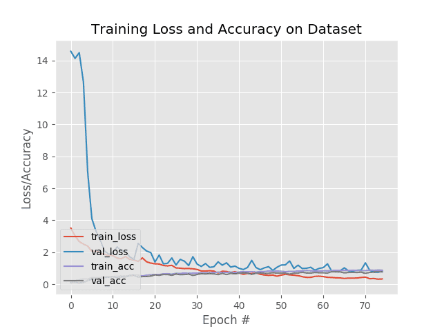
As a final step, we’ll use our training history dictionary, H , to generate a plot with matplotlib:
# plot the training loss and accuracy
N = NUM_EPOCHS
plt.style.use("ggplot")
plt.figure()
plt.plot(np.arange(0, N), H.history["loss"], label="train_loss")
plt.plot(np.arange(0, N), H.history["val_loss"], label="val_loss")
plt.plot(np.arange(0, N), H.history["accuracy"], label="train_acc")
plt.plot(np.arange(0, N), H.history["val_accuracy"], label="val_acc")
plt.title("Training Loss and Accuracy on Dataset")
plt.xlabel("Epoch #")
plt.ylabel("Loss/Accuracy")
plt.legend(loc="lower left")
plt.savefig("plot.png")
The accuracy/loss plot is generated and saved to disk as plot.png for inspection upon script exit.
Training a Keras model using fit_generator and evaluating with predict_generator
2020-06-03 Update: Despite the heading to this section, we now use .fit (sans .fit_generator) and .predict (sans .predict_generator).
To train our Keras model using our custom data generator, make sure you use the “Downloads” section to download the source code and example CSV image dataset.
From there, open a terminal, navigate to where you downloaded the source code + dataset, and execute the following command:
$ python train.py
Using TensorFlow backend.
[INFO] training w/ generator...
Train for 31 steps, validate for 10 steps
Epoch 1/75
31/31 [==============================] - 10s 317ms/step - loss: 3.6791 - accuracy: 0.1401 - val_loss: 1828.6441 - val_accuracy: 0.0625
Epoch 2/75
31/31 [==============================] - 9s 287ms/step - loss: 3.0351 - accuracy: 0.2077 - val_loss: 246.5172 - val_accuracy: 0.0938
Epoch 3/75
31/31 [==============================] - 9s 288ms/step - loss: 2.8571 - accuracy: 0.2621 - val_loss: 92.0763 - val_accuracy: 0.0750
...
31/31 [==============================] - 9s 287ms/step - loss: 0.4484 - accuracy: 0.8548 - val_loss: 1.3388 - val_accuracy: 0.6531
Epoch 73/75
31/31 [==============================] - 9s 287ms/step - loss: 0.4025 - accuracy: 0.8619 - val_loss: 1.1642 - val_accuracy: 0.7125
Epoch 74/75
31/31 [==============================] - 9s 287ms/step - loss: 0.3401 - accuracy: 0.8720 - val_loss: 1.2229 - val_accuracy: 0.7188
Epoch 75/75
31/31 [==============================] - 9s 287ms/step - loss: 0.3605 - accuracy: 0.8780 - val_loss: 1.2207 - val_accuracy: 0.7063
[INFO] evaluating network...
              precision    recall  f1-score   support

    bluebell       0.63      0.81      0.71        21
   buttercup       0.69      0.73      0.71        15
   coltsfoot       0.55      0.76      0.64        21
     cowslip       0.73      0.40      0.52        20
      crocus       0.53      0.88      0.66        24
    daffodil       0.82      0.33      0.47        27
       daisy       0.77      0.94      0.85        18
   dandelion       0.71      0.83      0.77        18
  fritillary       1.00      0.77      0.87        22
        iris       0.95      0.75      0.84        24
  lilyvalley       0.92      0.55      0.69        22
       pansy       0.89      0.89      0.89        18
    snowdrop       0.69      0.50      0.58        22
   sunflower       0.90      1.00      0.95        18
   tigerlily       0.87      0.93      0.90        14
       tulip       0.33      0.50      0.40        16
  windflower       0.81      0.85      0.83        20

    accuracy                           0.72       340
   macro avg       0.75      0.73      0.72       340
weighted avg       0.76      0.72      0.71       340
Here you can see that our network has obtained 76% accuracy on the evaluation set, which is quite respectable for the relatively shallow CNN used.
Most importantly, you learned how to utilize:
- Data generators
.fit(formerly.fit_generator).predict(formerly.predict_generator)
…all to train and evaluate your own custom Keras model!
Again, it’s not the actual format of the data itself that’s important here. Instead of CSV files, we could have been working with Caffe or TensorFlow record files, a combination of numerical/categorical data along with images, or any other synthesis of data that you may encounter in the real-world.
Instead, it’s the actual process of implementing your own Keras data generator that matters here.
Follow the steps in this tutorial and you’ll have a blueprint that you can use for implementing your own Keras data generators.
If you’re using TensorFlow 2.2+, just use “.fit”, there’s no reason to use “.fit_generator”
You can check your TensorFlow version by using pip freeze and then looking for your TensorFlow version:
$ pip freeze | grep 'tensorflow'
tensorflow==2.4.1
tensorflow-estimator==2.4.0
Provided you are using TensorFlow 2.2 or greater, you should just be using the .fit method.
TensorFlow will be deprecating the .fit_generator method in future releases as the .fit method can automatically detect whether or not the input data is an array or a generator.
What's next? We recommend PyImageSearch University.
86+ total classes • 115+ hours hours of on-demand code walkthrough videos • Last updated: April 2026
★★★★★ 4.84 (128 Ratings) • 16,000+ Students Enrolled
I strongly believe that if you had the right teacher you could master computer vision and deep learning.
Do you think learning computer vision and deep learning has to be time-consuming, overwhelming, and complicated? Or has to involve complex mathematics and equations? Or requires a degree in computer science?
That’s not the case.
All you need to master computer vision and deep learning is for someone to explain things to you in simple, intuitive terms. And that’s exactly what I do. My mission is to change education and how complex Artificial Intelligence topics are taught.
If you're serious about learning computer vision, your next stop should be PyImageSearch University, the most comprehensive computer vision, deep learning, and OpenCV course online today. Here you’ll learn how to successfully and confidently apply computer vision to your work, research, and projects. Join me in computer vision mastery.
Inside PyImageSearch University you'll find:
- ✓ 86+ courses on essential computer vision, deep learning, and OpenCV topics
- ✓ 86 Certificates of Completion
- ✓ 115+ hours hours of on-demand video
- ✓ Brand new courses released regularly, ensuring you can keep up with state-of-the-art techniques
- ✓ Pre-configured Jupyter Notebooks in Google Colab
- ✓ Run all code examples in your web browser — works on Windows, macOS, and Linux (no dev environment configuration required!)
- ✓ Access to centralized code repos for all 540+ tutorials on PyImageSearch
- ✓ Easy one-click downloads for code, datasets, pre-trained models, etc.
- ✓ Access on mobile, laptop, desktop, etc.
Summary
In this tutorial you learned the differences between Keras’ three primary functions used to train a deep neural network:
.fit: Used when the entire training dataset can fit into memory and no data augmentation is applied. As of TensorFlow 2, this method now supports data augmentation..fit_generator: For legacy code using versions of TensorFlow/Keras prior to 2.2. Should be used when either (1) the dataset is too large to fit into memory, (2) data augmentation needs to be applied, or (3) in any situation when it’s more convenient to yield training data in batches (i.e., using theflow_from_directoryfunction)..train_on_batch: Can be used to train a Keras model on a single batch of data. Should be utilized only when you need the finest-grained control training your network, such as in situations where your data iterator is highly complex.
From there, we discovered how to:
- Implement our own custom Keras generator function
- Use our custom generator along with Keras’
.fit_generatorto train our deep neural network
You can use today’s example code as a template when implementing your own Keras generators in your own projects.
I hope you enjoyed today’s blog post!
To download the source code to this post, and be notified when future tutorials are published here on PyImageSearch, just enter your email address in the form below!

Download the Source Code and FREE 17-page Resource Guide
Enter your email address below to get a .zip of the code and a FREE 17-page Resource Guide on Computer Vision, OpenCV, and Deep Learning. Inside you'll find my hand-picked tutorials, books, courses, and libraries to help you master CV and DL!
