Inside this Keras tutorial, you will discover how easy it is to get started with deep learning and Python. You will use the Keras deep learning library to train your first neural network on a custom image dataset, and from there, you’ll implement your first Convolutional Neural Network (CNN) as well.
The inspiration for this guide came from PyImageSearch reader, Igor, who emailed me a few weeks ago and asked:
Hey Adrian, thanks for the PyImageSearch blog. I’ve noticed that nearly every “getting started” guide I come across for Keras and image classification uses either the MNIST or CIFAR-10 datasets which are built into Keras. I just call one of those functions and the data is automatically loaded for me.
But how do I go about using my own image dataset with Keras?
What steps do I have to take?
Igor has a great point — most Keras tutorials you come across will try to teach you the basics of the library using an image classification dataset such MNIST (handwriting recognition) or CIFAR-10 (basic object recognition).
These image datasets are standard benchmarks in the computer vision and deep learning literature, and sure, they will absolutely get you started using Keras…
…but they aren’t necessarily practical in the sense that they don’t teach you how to work with your own set of images residing on disk. Instead, you’re just calling helper functions to load pre-compiled datasets.
I’m going with a different take on an introductory Keras tutorial.
Instead of teaching you how to utilize one of these pre-compiled datasets, I’m going to teach you how to train your first neural network and Convolutional Neural Network using a custom dataset — because let’s face it, your goal is to apply deep learning to your own dataset, not one built into Keras, am I right?
To learn how to get started with Keras, Deep Learning, and Python, just keep reading!
Keras Tutorial: How to get started with Keras, Deep Learning, and Python
2020-05-13 Update: This blog post is now TensorFlow 2+ compatible!
Today’s Keras tutorial is designed with the practitioner in mind — it is meant to be a practitioner’s approach to applied deep learning.
That means that we’ll learn by doing.
We’ll be getting our hands dirty.
Writing some Keras code.
And then training our networks on our custom datasets.
This tutorial is not meant to be a deep dive into the theory surrounding deep learning.
If you’re interested in studying deep learning in odepth, including both (1) hands-on implementations and (2) a discussion of theory, I would suggest you check out my book, Deep Learning for Computer Vision with Python.
Overview of what’s going to be covered
Training your first simple neural network with Keras doesn’t require a lot of code, but we’re going to start slow, taking it step-by-step, ensuring you understand the process of how to train a network on your own custom dataset.
The steps we’ll cover today include:
- Installing Keras and other dependencies on your system
- Loading your data from disk
- Creating your training and testing splits
- Defining your Keras model architecture
- Compiling your Keras model
- Training your model on your training data
- Evaluating your model on your test data
- Making predictions using your trained Keras model
I’ve also included an additional section on training your first Convolutional Neural Network.
This may seem like a lot of steps, but I promise you, once we start getting into the example you’ll see that the examples are linear, make intuitive sense, and will help you understand the fundamentals of training a neural network with Keras.
Our example dataset
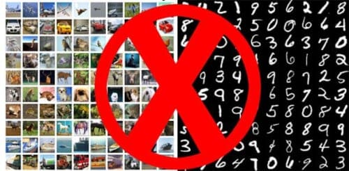
Most Keras tutorials you come across for image classification will utilize MNIST or CIFAR-10 — I’m not going to do that here.
To start, MNIST and CIFAR-10 aren’t very exciting examples.
These tutorials don’t actually cover how to work with your own custom image datasets. Instead, they simply call built-in Keras utilities that magically return the MNIST and CIFAR-10 datasets as NumPy arrays. In fact, your training and testing splits have already been pre-split for you!
Secondly, if you want to use your own custom datasets you really don’t know where to start. You’ll find yourself scratching your head and asking questions such as:
- Where are those helper functions loading the data from?
- What format should my dataset on disk be?
- How can I load my dataset into memory?
- What preprocessing steps do I need to perform?
Let’s be honest — your goal in studying Keras and deep learning isn’t to work with these pre-baked datasets.
Instead, you want to work with your own custom datasets.
And those introductory Keras tutorials you’ve come across only take you so far.
That’s why, inside this Keras tutorial, we’ll be working with a custom dataset called the “Animals dataset” I created for my book, Deep Learning for Computer Vision with Python:

The purpose of this dataset is to correctly classify an image as containing either:
- Cats
- Dogs
- Pandas
Containing only 3,000 images, the Animals dataset is meant to be an introductory dataset that we can quickly train a deep learning model on using either our CPU or GPU (and still obtain reasonable accuracy).
Furthermore, using this custom dataset enables you to understand:
- How you should organize your dataset on disk
- How to load your images and class labels from disk
- How to partition your data into training and testing splits
- How to train your first Keras neural network on the training data
- How to evaluate your model on the testing data
- How you can reuse your trained model on data that is brand new and outside your training and testing splits
By following the steps in this Keras tutorial you’ll be able to swap out my Animals dataset for any dataset of your choice, provided you utilize the project/directory structure detailed below.
Need data? If you need to scrape images from the internet to create a dataset, check out how to do it the easy way with Bing Image Search, or the slightly more involved way with Google Images.
Project structure
There are a number of files associated with this project. Grab the zip from the “Downloads” section and then use the tree command to show the project structure in your terminal (I’ve provided two command line argument flags to tree to make the output nice and clean):
$ tree --dirsfirst --filelimit 10
.
├── animals
│   ├── cats [1000 entries exceeds filelimit, not opening dir]
│   ├── dogs [1000 entries exceeds filelimit, not opening dir]
│   └── panda [1000 entries exceeds filelimit, not opening dir]
├── images
│   ├── cat.jpg
│   ├── dog.jpg
│   └── panda.jpg
├── output
│   ├── simple_nn.model
│   ├── simple_nn_lb.pickle
│   ├── simple_nn_plot.png
│   ├── smallvggnet.model
│   ├── smallvggnet_lb.pickle
│   └── smallvggnet_plot.png
├── pyimagesearch
│   ├── __init__.py
│   └── smallvggnet.py
├── predict.py
├── train_simple_nn.py
└── train_vgg.py

7 directories, 14 files
As previously discussed, today we’ll be working with the Animals dataset. Notice how animals is organized in the project tree. Inside of animals/ , there are three class directories: cats/ , dogs/ , panda/ . Within each of those directories is 1,000 images pertaining to the respective class.
If you work with your own dataset, just organize it the same way! Ideally you’ll gather 1,000 images per class at a minimum. This isn’t always possible, but you should at least have class balance. Significantly more images in one class folder could cause model bias.
Next is the images/ directory. This directory contains three images for testing purposes which we’ll use to demonstrate how to (1) load a trained model from disk and then (2) classify an input image that is not part of our original dataset.
The output/ folder contains three types of files which are generated by training:
.model: A serialized Keras model file is generated after training and can be used in future inference scripts..pickle: A serialized label binarizer file. This file contains an object which contains class names. It accompanies a model file..png: I always place my training/validation plot images in the output folder as it is an output of the training process.
The pyimagesearch/ directory is a module. Contrary to the many questions I receive, pyimagesearch is not a pip-installable package. Instead it resides in the project folder and classes contained within can be imported into your scripts. It is provided in the “Downloads” section of this Keras tutorial.
Today we’ll be reviewing four .py files:
- In the first half of the blog post, we’ll train a simple model. The training script is
train_simple_nn.py. - We’ll advance to training
SmallVGGNetusing thetrain_vgg.pyscript. - The
smallvggnet.pyfile contains ourSmallVGGNetclass, a Convolutional Neural Network. - What good is a serialized model unless we can deploy it? In
predict.py, I’ve provided sample code for you to load a serialized model + label file and make an inference on an image. The prediction script is only useful after we have successfully trained a model with reasonable accuracy. It is always useful to run this script to test with images that are not contained within the dataset.
Configuring your development environment

To configure your system for this tutorial, I first recommend following either of these tutorials:
Either tutorial will help you configure you system with all the necessary software for this blog post in a convenient Python virtual environment.
Please note that PyImageSearch does not recommend or support Windows for CV/DL projects.
2. Load your data from disk

Now that Keras is installed on our system we can start implementing our first simple neural network training script using Keras. We’ll later implement a full-blown Convolutional Neural Network, but let’s start easy and work our way up.
Open up train_simple_nn.py and insert the following code:
# set the matplotlib backend so figures can be saved in the background
import matplotlib
matplotlib.use("Agg")

# import the necessary packages
from sklearn.preprocessing import LabelBinarizer
from sklearn.model_selection import train_test_split
from sklearn.metrics import classification_report
from tensorflow.keras.models import Sequential
from tensorflow.keras.layers import Dense
from tensorflow.keras.optimizers import SGD
from imutils import paths
import matplotlib.pyplot as plt
import numpy as np
import argparse
import random
import pickle
import cv2
import os
Lines 2-19 import our required packages. As you can see there are quite a few tools this script is taking advantage of. Let’s review the important ones:
matplotlib: This is the go-to plotting package for Python. That said, it does have its nuances, and if you’re having trouble with it, refer to this blog post. On Line 3, we instructmatplotlibto use the"Agg"backend enabling us to save plots to disk — that’s your first nuance!sklearn: The scikit-learn library will help us with binarizing our labels, splitting data for training/testing, and generating a training report in our terminal.tensorflow.keras: You’re reading this tutorial to learn about Keras — it is our high level frontend into TensorFlow and other deep learning backends.imutils: My package of convenience functions. We’ll use thepathsmodule to generate a list of image file paths for training.numpy: NumPy is for numerical processing with Python. It is another go-to package. If you have OpenCV for Python and scikit-learn installed, then you’ll have NumPy as it is a dependency.cv2: This is OpenCV. At this point, it is both tradition and a requirement to tack on the 2 even though you’re likely using OpenCV 3 or higher.- …the remaining imports are built into your installation of Python!
Wheww! That was a lot, but having a good idea of what each import is used for will aid your understanding as we walk through these scripts.
Let’s parse our command line arguments with argparse:
# construct the argument parser and parse the arguments
ap = argparse.ArgumentParser()
ap.add_argument("-d", "--dataset", required=True,
	help="path to input dataset of images")
ap.add_argument("-m", "--model", required=True,
	help="path to output trained model")
ap.add_argument("-l", "--label-bin", required=True,
	help="path to output label binarizer")
ap.add_argument("-p", "--plot", required=True,
	help="path to output accuracy/loss plot")
args = vars(ap.parse_args())
Our script will dynamically handle additional information provided via the command line when we execute our script. The additional information is in the form of command line arguments. The argparse module is built into Python and will handle parsing the information you provide in your command string. For additional explanation, refer to this blog post.
We have four command line arguments to parse:
--dataset: The path to our dataset of images on disk.--model: Our model will be serialized and output to disk. This argument contains the path to the output model file.--label-bin: Dataset labels are serialized to disk for easy recall in other scripts. This is the path to the output label binarizer file.--plot: The path to the output training plot image file. We’ll review this plot to check for over/underfitting of our data.
With the dataset information in hand, let’s load our images and class labels:
# initialize the data and labels
print("[INFO] loading images...")
data = []
labels = []

# grab the image paths and randomly shuffle them
imagePaths = sorted(list(paths.list_images(args["dataset"])))
random.seed(42)
random.shuffle(imagePaths)

# loop over the input images
for imagePath in imagePaths:
	# load the image, resize the image to be 32x32 pixels (ignoring
	# aspect ratio), flatten the image into 32x32x3=3072 pixel image
	# into a list, and store the image in the data list
	image = cv2.imread(imagePath)
	image = cv2.resize(image, (32, 32)).flatten()
	data.append(image)

	# extract the class label from the image path and update the
	# labels list
	label = imagePath.split(os.path.sep)[-2]
	labels.append(label)
Here we:
- Initialize lists for our
dataandlabels(Lines 35 and 36). These will later become NumPy arrays. - Grab
imagePathsand randomly shuffle them (Lines 39-41). Thepaths.list_imagesfunction conveniently will find all the paths to all input images in our--datasetdirectory before we sort andshufflethem. I set aseedso that the random reordering is reproducible. - Begin looping over all
imagePathsin our dataset (Line 44).
For each imagePath , we proceed to:
- Load the
imageinto memory (Line 48). - Resize the
imageto32x32pixels (ignoring aspect ratio) as well asflattenthe image (Line 49). It is critical toresizeour images properly because this neural network requires these dimensions. Each neural network will require different dimensions, so just be aware of this. Flattening the data allows us to pass the raw pixel intensities to the input layer neurons easily. You’ll see later that for VGGNet we pass the volume to the network since it is convolutional. Keep in mind that this example is just a simple non-convolutional network — we’ll be looking at a more advanced example later in the post. - Append the resized image to
data(Line 50). - Extract the class
labelof the image from the path (Line 54) and add it to thelabelslist (Line 55). Thelabelslist contains the classes that correspond to each image in the data list.
Now in one fell swoop, we can apply array operations to the data and labels:
# scale the raw pixel intensities to the range [0, 1]
data = np.array(data, dtype="float") / 255.0
labels = np.array(labels)
On Line 58 we scale pixel intensities from the range [0, 255] to [0, 1] (a common preprocessing step).
We also convert the labels list to a NumPy array (Line 59).
3. Construct your training and testing splits
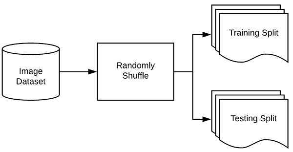
Now that we have loaded our image data from disk, next we need to construct our training and testing splits:
# partition the data into training and testing splits using 75% of
# the data for training and the remaining 25% for testing
(trainX, testX, trainY, testY) = train_test_split(data,
	labels, test_size=0.25, random_state=42)
It is typical to allocate a percentage of your data for training and a smaller percentage of your data for testing. The scikit-learn provides a handy train_test_split function which will split the data for us.
Both trainX and testX make up the image data itself while trainY and testY make up the labels.
Our class labels are currently represented as strings; however, Keras will assume that both:
- Labels are encoded as integers
- And furthermore, one-hot encoding is performed on these labels making each label represented as a vector rather than an integer
To accomplish this encoding, we can use the LabelBinarizer class from scikit-learn:
# convert the labels from integers to vectors (for 2-class, binary
# classification you should use Keras' to_categorical function
# instead as the scikit-learn's LabelBinarizer will not return a
# vector)
lb = LabelBinarizer()
trainY = lb.fit_transform(trainY)
testY = lb.transform(testY)
On Line 70, we initialize the LabelBinarizer object.
A call to fit_transform finds all unique class labels in trainY and then transforms them into one-hot encoded labels.
A call to just .transform on testY performs just the one-hot encoding step — the unique set of possible class labels was already determined by the call to .fit_transform .
Here’s an example:
[1, 0, 0] # corresponds to cats
[0, 1, 0] # corresponds to dogs
[0, 0, 1] # corresponds to panda
Notice how only one of the array elements is “hot” which is why we call this “one-hot” encoding.
4. Define your Keras model architecture
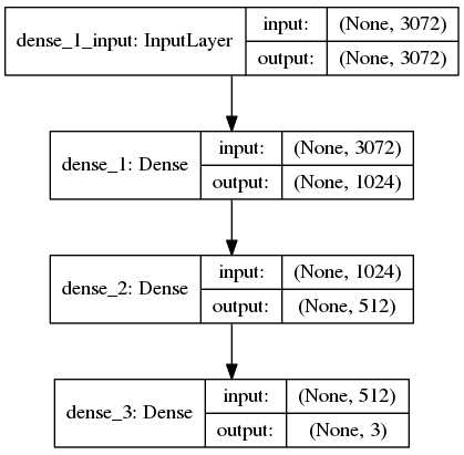
The next step is to define our neural network architecture using Keras. Here we will be using a network with one input layer, two hidden layers, and one output layer:
# define the 3072-1024-512-3 architecture using Keras
model = Sequential()
model.add(Dense(1024, input_shape=(3072,), activation="sigmoid"))
model.add(Dense(512, activation="sigmoid"))
model.add(Dense(len(lb.classes_), activation="softmax"))
Since our model is really simple, we go ahead and define it in this script (typically I like to make a separate class in a separate file for the model architecture).
The input layer and first hidden layer are defined on Line 76. will have an input_shape of 3072 as there are 32x32x3=3072 pixels in a flattened input image. The first hidden layer will have 1024 nodes.
The second hidden layer will have 512 nodes (Line 77).
Finally, the number of nodes in the final output layer (Line 78) will be the number of possible class labels — in this case, the output layer will have three nodes, one for each of our class labels (“cats”, “dogs”, and “panda”, respectively).
5. Compile your Keras model
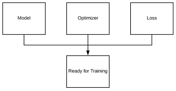
Once we have defined our neural network architecture, the next step is to “compile” it:
# initialize our initial learning rate and # of epochs to train for
INIT_LR = 0.01
EPOCHS = 80

# compile the model using SGD as our optimizer and categorical
# cross-entropy loss (you'll want to use binary_crossentropy
# for 2-class classification)
print("[INFO] training network...")
opt = SGD(lr=INIT_LR)
model.compile(loss="categorical_crossentropy", optimizer=opt,
	metrics=["accuracy"])
First, we initialize our learning rate and total number of epochs to train for (Lines 81 and 82).
Then we compile our model using the Stochastic Gradient Descent (SGD ) optimizer with "categorical_crossentropy" as the loss function.
Categorical cross-entropy is used as the loss for nearly all networks trained to perform classification. The only exception is for 2-class classification where there are only two possible class labels. In that event you would want to swap out "categorical_crossentropy" for "binary_crossentropy" .
6. Fit your Keras model to the data

Now that our Keras model is compiled, we can “fit” (i.e., train) it on our training data:
# train the neural network
H = model.fit(x=trainX, y=trainY, validation_data=(testX, testY),
	epochs=EPOCHS, batch_size=32)
We’ve discussed all the inputs except batch_size . The batch_size controls the size of each group of data to pass through the network. Larger GPUs would be able to accommodate larger batch sizes. I recommend starting with 32 or 64 and going up from there.
7. Evaluate your Keras model

We’ve trained our actual model but now we need to evaluate it on our testing data.
It’s important that we evaluate on our testing data so we can obtain an unbiased (or as close to unbiased as possible) representation of how well our model is performing with data it has never been trained on.
To evaluate our Keras model we can use a combination of the .predict method of the model along with the classification_report from scikit-learn:
# evaluate the network
print("[INFO] evaluating network...")
predictions = model.predict(x=testX, batch_size=32)
print(classification_report(testY.argmax(axis=1),
	predictions.argmax(axis=1), target_names=lb.classes_))

# plot the training loss and accuracy
N = np.arange(0, EPOCHS)
plt.style.use("ggplot")
plt.figure()
plt.plot(N, H.history["loss"], label="train_loss")
plt.plot(N, H.history["val_loss"], label="val_loss")
plt.plot(N, H.history["accuracy"], label="train_acc")
plt.plot(N, H.history["val_accuracy"], label="val_acc")
plt.title("Training Loss and Accuracy (Simple NN)")
plt.xlabel("Epoch #")
plt.ylabel("Loss/Accuracy")
plt.legend()
plt.savefig(args["plot"])
2020-05-13 Update: In order for this plotting snippet to be TensorFlow 2+ compatible the H.history dictionary keys are updated to fully spell out “accuracy” sans “acc” (i.e., H.history["val_accuracy"] and H.history["accuracy"]). It is semi-confusing that “val” is not spelled out as “validation”; we have to learn to love and live with the API and always remember that it is a work in progress that many developers around the world contribute to.
When running this script you’ll notice that our Keras neural network will start to train, and once training is complete, we’ll evaluate the network on our testing set:
$ python train_simple_nn.py --dataset animals --model output/simple_nn.model \
	--label-bin output/simple_nn_lb.pickle --plot output/simple_nn_plot.png
Using TensorFlow backend.
[INFO] loading images...
[INFO] training network...
Train on 2250 samples, validate on 750 samples
Epoch 1/80
2250/2250 [==============================] - 1s 311us/sample - loss: 1.1041 - accuracy: 0.3516 - val_loss: 1.1578 - val_accuracy: 0.3707
Epoch 2/80
2250/2250 [==============================] - 0s 183us/sample - loss: 1.0877 - accuracy: 0.3738 - val_loss: 1.0766 - val_accuracy: 0.3813
Epoch 3/80
2250/2250 [==============================] - 0s 181us/sample - loss: 1.0707 - accuracy: 0.4240 - val_loss: 1.0693 - val_accuracy: 0.3533
...
Epoch 78/80
2250/2250 [==============================] - 0s 184us/sample - loss: 0.7688 - accuracy: 0.6160 - val_loss: 0.8696 - val_accuracy: 0.5880
Epoch 79/80
2250/2250 [==============================] - 0s 181us/sample - loss: 0.7675 - accuracy: 0.6200 - val_loss: 1.0294 - val_accuracy: 0.5107
Epoch 80/80
2250/2250 [==============================] - 0s 181us/sample - loss: 0.7687 - accuracy: 0.6164 - val_loss: 0.8361 - val_accuracy: 0.6120
[INFO] evaluating network...
              precision    recall  f1-score   support

        cats       0.57      0.59      0.58       236
        dogs       0.55      0.31      0.39       236
       panda       0.66      0.89      0.76       278

    accuracy                           0.61       750
   macro avg       0.59      0.60      0.58       750
weighted avg       0.60      0.61      0.59       750

[INFO] serializing network and label binarizer...
This network is small, and when combined with a small dataset, takes only 2 seconds per epoch on my CPU.
Here you can see that our network is obtaining 60% accuracy.
Since we would have a 1/3 chance of randomly picking the correct label for a given image we know that our network has actually learned patterns that can be used to discriminate between the three classes.
We also save a plot of our:
- Training loss
- Validation loss
- Training accuracy
- Validation accuracy
…ensuring that we can easily spot overfitting or underfitting in our results.
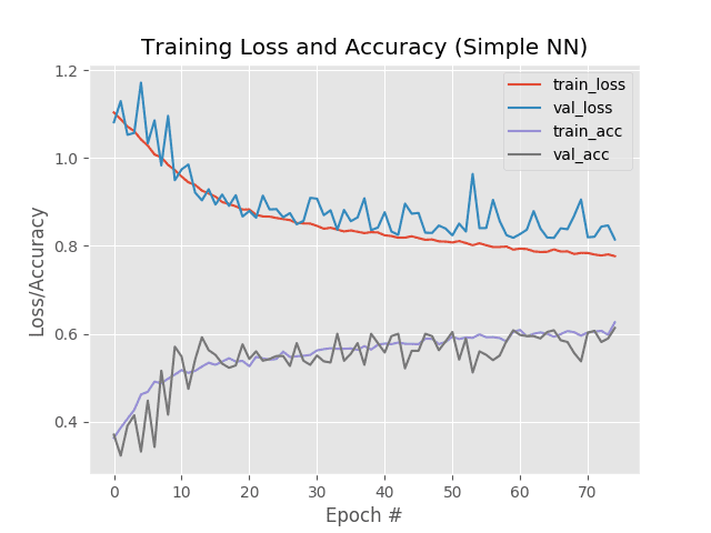
Looking at our plot we see a small amount of overfitting start to occur past epoch ~45 where our training and validation losses start to diverge and a pronounced gap appears.
Finally, we can save our model to disk so we can reuse it later without having to retrain it:
# save the model and label binarizer to disk
print("[INFO] serializing network and label binarizer...")
model.save(args["model"], save_format="h5")
f = open(args["label_bin"], "wb")
f.write(pickle.dumps(lb))
f.close()
8. Make predictions on new data using your Keras model
At this point our model is trained — but what if we wanted to make predictions on images after our network has already been trained?
What would we do then?
How would we load the model from disk?
How can we load an image and then preprocess it for classification?
Inside the predict.py script, I’ll show you how, so open it and insert the following code:
# import the necessary packages
from tensorflow.keras.models import load_model
import argparse
import pickle
import cv2

# construct the argument parser and parse the arguments
ap = argparse.ArgumentParser()
ap.add_argument("-i", "--image", required=True,
	help="path to input image we are going to classify")
ap.add_argument("-m", "--model", required=True,
	help="path to trained Keras model")
ap.add_argument("-l", "--label-bin", required=True,
	help="path to label binarizer")
ap.add_argument("-w", "--width", type=int, default=28,
	help="target spatial dimension width")
ap.add_argument("-e", "--height", type=int, default=28,
	help="target spatial dimension height")
ap.add_argument("-f", "--flatten", type=int, default=-1,
	help="whether or not we should flatten the image")
args = vars(ap.parse_args())
First, we’ll import our required packages and modules.
You’ll need to explicitly import load_model from tensorflow.keras.models whenever you write a script to load a Keras model from disk. OpenCV will be used for annotation and display. The pickle module will be used to load our label binarizer.
Next, let’s parse our command line arguments:
--image: The path to our input image.--model: Our trained and serialized Keras model path.--label-bin: Path to the serialized label binarizer.--width: The width of the input shape for our CNN. Remember — you can’t just specify anything here. You need to specify the width that the model is designed for.--height: The height of the image input to the CNN. The height specified must also match the network’s input shape.--flatten: Whether or not we should flatten the image. By default, we won’t flatten the image. If you need to flatten the image, you should pass a1for this argument.
Next, let’s load the image and resize it based on the command line arguments:
# load the input image and resize it to the target spatial dimensions
image = cv2.imread(args["image"])
output = image.copy()
image = cv2.resize(image, (args["width"], args["height"]))

# scale the pixel values to [0, 1]
image = image.astype("float") / 255.0
And then we’ll flatten the image if necessary:
# check to see if we should flatten the image and add a batch
# dimension
if args["flatten"] > 0:
	image = image.flatten()
	image = image.reshape((1, image.shape[0]))

# otherwise, we must be working with a CNN -- don't flatten the
# image, simply add the batch dimension
else:
	image = image.reshape((1, image.shape[0], image.shape[1],
		image.shape[2]))
Flattening the image for standard fully-connected networks is straightforward (Lines 33-35).
In the case of a CNN, we also add the batch dimension, but we do not flatten the image (Lines 39-41). An example CNN is covered in the next section.
From there, let’s load the model + label binarizer into memory and make a prediction:
# load the model and label binarizer
print("[INFO] loading network and label binarizer...")
model = load_model(args["model"])
lb = pickle.loads(open(args["label_bin"], "rb").read())

# make a prediction on the image
preds = model.predict(image)

# find the class label index with the largest corresponding
# probability
i = preds.argmax(axis=1)[0]
label = lb.classes_[i]
Our model and label binarizer are loaded via Lines 45 and 46.
We can make predictions on the input image by calling model.predict (Line 49).
What does the preds array look like?
(Pdb) preds
array([[5.4622066e-01, 4.5377851e-01, 7.7963534e-07]], dtype=float32)
The 2D array contains (1) the index of the image in the batch (here there is only one index as there was only one image passed into the NN for classification) and (2) percentages corresponding to each class label, as shown by querying the variable in my Python debugger:
- cats: 54.6%
- dogs: 45.4%
- panda: ~0%
In other words, our network “thinks” that it sees “cats” and it sure as hell “knows” that it doesn’t see a “panda”.
Line 53 finds the index of the max value (the 0-th “cats” index).
And Line 54 extracts the “cats” string label from the label binarizer.
Easy right?
Now let’s display the results:
# draw the class label + probability on the output image
text = "{}: {:.2f}%".format(label, preds[0][i] * 100)
cv2.putText(output, text, (10, 30), cv2.FONT_HERSHEY_SIMPLEX, 0.7,
	(0, 0, 255), 2)

# show the output image
cv2.imshow("Image", output)
cv2.waitKey(0)
We format our text string on Line 57. This includes the label and the prediction value in percentage format.
Then we place the text on the output image (Lines 58 and 59).
Finally, we show the output image on the screen and wait until the user presses any key on Lines 62 and 63 (watch Homer Simpson try to locate the “any” key).
Our prediction script was rather straightforward.
Once you’ve used the “Downloads” section of this tutorial to download the code, you can open up a terminal and try running our trained network on custom images:
$ python predict.py --image images/cat.jpg --model output/simple_nn.model \
	--label-bin output/simple_nn_lb.pickle --width 32 --height 32 --flatten 1
Using TensorFlow backend.
[INFO] loading network and label binarizer...
Be sure that you copy/pasted or typed the entire command (including command line arguments) from within the folder relative to the script. If you’re having trouble with the command line arguments, give this blog post a read.
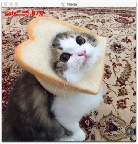
Here you can see that our simple Keras neural network has classified the input image as “cats” with 55.87% probability, despite the cat’s face being partially obscured by a piece of bread.
9. BONUS: Training your first Convolutional Neural Network with Keras
Admittedly, using a standard feedforward neural network to classify images is not a wise choice.
Instead, we should leverage Convolutional Neural Networks (CNNs) which are designed to operate over the raw pixel intensities of images and learn discriminating filters that can be used to classify images with high accuracy.
The model we’ll be discussing here today is a smaller variant of VGGNet which I have named “SmallVGGNet”.
VGGNet-like models share two common characteristics:
- Only 3×3 convolutions are used
- Convolution layers are stacked on top of each other deeper in the network architecture prior to applying a destructive pooling operation
Let’s go ahead and implement SmallVGGNet now.
Open up the smallvggnet.py file and insert the following code:
# import the necessary packages
from tensorflow.keras.models import Sequential
from tensorflow.keras.layers import BatchNormalization
from tensorflow.keras.layers import Conv2D
from tensorflow.keras.layers import MaxPooling2D
from tensorflow.keras.layers import Activation
from tensorflow.keras.layers import Flatten
from tensorflow.keras.layers import Dropout
from tensorflow.keras.layers import Dense
from tensorflow.keras import backend as K
As you can see from the imports on Lines 2-10, everything needed for the SmallVGGNet comes from keras . I encourage you to familiarize yourself with each in the Keras documentation and in my deep learning book.
We then begin to define our SmallVGGNet class and the build method:
class SmallVGGNet:
	@staticmethod
	def build(width, height, depth, classes):
		# initialize the model along with the input shape to be
		# "channels last" and the channels dimension itself
		model = Sequential()
		inputShape = (height, width, depth)
		chanDim = -1

		# if we are using "channels first", update the input shape
		# and channels dimension
		if K.image_data_format() == "channels_first":
			inputShape = (depth, height, width)
			chanDim = 1
Our class is defined on Line 12 and the sole build method is defined on Line 14.
Four parameters are required for build : the width of the input images, the height of the height input images, the depth , and number of classes .
The depth can also be thought of as the number of channels. Our images are in the RGB color space, so we’ll pass a depth of 3 when we call the build method.
First, we initialize a Sequential model (Line 17).
Then, we determine channel ordering. Keras supports "channels_last" (i.e. TensorFlow) and "channels_first" (i.e. Theano) ordering. Lines 18-25 allow our model to support either type of backend.
Now, let’s add some layers to the network:
		# CONV => RELU => POOL layer set
		model.add(Conv2D(32, (3, 3), padding="same",
			input_shape=inputShape))
		model.add(Activation("relu"))
		model.add(BatchNormalization(axis=chanDim))
		model.add(MaxPooling2D(pool_size=(2, 2)))
		model.add(Dropout(0.25))
Our first CONV => RELU => POOL layers are added by this block.
Our first CONV layer has 32 filters of size 3x3 .
It is very important that we specify the inputShape for the first layer as all subsequent layer dimensions will be calculated using a trickle-down approach.
We’ll use the ReLU (Rectified Linear Unit) activation function in this network architecture. There are a number of activation methods and I encourage you to familiarize yourself with the popular ones inside Deep Learning for Computer Vision with Python where pros/cons and tradeoffs are discussed.
Batch Normalization, MaxPooling, and Dropout are also applied.
Batch Normalization is used to normalize the activations of a given input volume before passing it to the next layer in the network. It has been proven to be very effective at reducing the number of epochs required to train a CNN as well as stabilizing training itself.
POOL layers have a primary function of progressively reducing the spatial size (i.e. width and height) of the input volume to a layer. It is common to insert POOL layers between consecutive CONV layers in a CNN architecture.
Dropout is an interesting concept not to be overlooked. In an effort to force the network to be more robust we can apply dropout, the process of disconnecting random neurons between layers. This process is proven to reduce overfitting, increase accuracy, and allow our network to generalize better for unfamiliar images. As denoted by the parameter, 25% of the node connections are randomly disconnected (dropped out) between layers during each training iteration.
Note: If you’re new to deep learning, this may all sound like a different language to you. Just like learning a new spoken language, it takes time, study, and practice. If you’re yearning to learn the language of deep learning, why not grab my highly rated book, Deep Learning for Computer Vision with Python? I promise that I break down these concepts in the book and reinforce them via practical examples.
Moving on, we reach our next block of (CONV => RELU) * 2 => POOL layers:
		# (CONV => RELU) * 2 => POOL layer set
		model.add(Conv2D(64, (3, 3), padding="same"))
		model.add(Activation("relu"))
		model.add(BatchNormalization(axis=chanDim))
		model.add(Conv2D(64, (3, 3), padding="same"))
		model.add(Activation("relu"))
		model.add(BatchNormalization(axis=chanDim))
		model.add(MaxPooling2D(pool_size=(2, 2)))
		model.add(Dropout(0.25))
Notice that our filter dimensions remain the same (3x3 , which is common for VGG-like networks); however, we’re increasing the total number of filters learned from 32 to 64.
This is followed by a (CONV => RELU => POOL) * 3 layer set:
		# (CONV => RELU) * 3 => POOL layer set
		model.add(Conv2D(128, (3, 3), padding="same"))
		model.add(Activation("relu"))
		model.add(BatchNormalization(axis=chanDim))
		model.add(Conv2D(128, (3, 3), padding="same"))
		model.add(Activation("relu"))
		model.add(BatchNormalization(axis=chanDim))
		model.add(Conv2D(128, (3, 3), padding="same"))
		model.add(Activation("relu"))
		model.add(BatchNormalization(axis=chanDim))
		model.add(MaxPooling2D(pool_size=(2, 2)))
		model.add(Dropout(0.25))
Again, notice how all CONV layers learn 3x3 filters but the total number of filters learned by the CONV layers has doubled from 64 to 128. Increasing the total number of filters learned the deeper you go into a CNN (and as your input volume size becomes smaller and smaller) is common practice.
And finally we have a set of FC => RELU layers:
		# first (and only) set of FC => RELU layers
		model.add(Flatten())
		model.add(Dense(512))
		model.add(Activation("relu"))
		model.add(BatchNormalization())
		model.add(Dropout(0.5))

		# softmax classifier
		model.add(Dense(classes))
		model.add(Activation("softmax"))

		# return the constructed network architecture
		return model
Fully connected layers are denoted by Dense in Keras. The final layer is fully connected with three outputs (since we have three classes in our dataset). The softmax layer returns the class probabilities for each label.
Now that SmallVGGNet is implemented, let’s write the driver script that will be used to train it on our Animals dataset.
Much of the code here will be similar to the previous example, but I’ll:
- Review the entire script as a matter of completeness
- And call out any differences along the way
Open up the train_vgg.py script and let’s get started:
# set the matplotlib backend so figures can be saved in the background
import matplotlib
matplotlib.use("Agg")

# import the necessary packages
from pyimagesearch.smallvggnet import SmallVGGNet
from sklearn.preprocessing import LabelBinarizer
from sklearn.model_selection import train_test_split
from sklearn.metrics import classification_report
from tensorflow.keras.preprocessing.image import ImageDataGenerator
from tensorflow.keras.optimizers import SGD
from imutils import paths
import matplotlib.pyplot as plt
import numpy as np
import argparse
import random
import pickle
import cv2
import os
The imports are the same as our previous training script with two exceptions:
- Instead of
from keras.models import Sequential, this time we importSmallVGGNetvia
from pyimagesearch.smallvggnet import SmallVGGNet. Scroll up slightly to see the SmallVGGNet implementation. - We will be augmenting our data with
ImageDataGenerator. Data augmentation is almost always recommended and leads to models that generalize better. Data augmentation involves adding applying random rotations, shifts, shears, and scaling to existing training data. You won’t see a bunch of new .png and .jpg files — it is done on the fly as the script executes.
You should recognize the other imports at this point. If not, just refer to the bulleted list above.
Let’s parse our command line arguments:
# construct the argument parser and parse the arguments
ap = argparse.ArgumentParser()
ap.add_argument("-d", "--dataset", required=True,
	help="path to input dataset of images")
ap.add_argument("-m", "--model", required=True,
	help="path to output trained model")
ap.add_argument("-l", "--label-bin", required=True,
	help="path to output label binarizer")
ap.add_argument("-p", "--plot", required=True,
	help="path to output accuracy/loss plot")
args = vars(ap.parse_args())
We have four command line arguments to parse:
--dataset: The path to our dataset of images on disk. This can be the path toanimals/or another dataset organized the same way.--model: Our model will be serialized and output to disk. This argument contains the path to the output model file. Be sure to name your model accordingly so you don’t overwrite any previously trained models (such as the simple neural network one).--label-bin: Dataset labels are serialized to disk for easy recall in other scripts. This is the path to the output label binarizer file.--plot: The path to the output training plot image file. We’ll review this plot to check for over/underfitting of our data. Each time you train your model with changes to parameters, you should specify a different plot filename in the command line so that you’ll have a history of plots corresponding to training notes in your notebook or notes file. This tutorial makes deep learning seem easy, but keep in mind that I went through several iterations of training before I settled on all parameters to share with you in this script.
Let’s load and preprocess our data:
# initialize the data and labels
print("[INFO] loading images...")
data = []
labels = []

# grab the image paths and randomly shuffle them
imagePaths = sorted(list(paths.list_images(args["dataset"])))
random.seed(42)
random.shuffle(imagePaths)

# loop over the input images
for imagePath in imagePaths:
	# load the image, resize it to 64x64 pixels (the required input
	# spatial dimensions of SmallVGGNet), and store the image in the
	# data list
	image = cv2.imread(imagePath)
	image = cv2.resize(image, (64, 64))
	data.append(image)

	# extract the class label from the image path and update the
	# labels list
	label = imagePath.split(os.path.sep)[-2]
	labels.append(label)

# scale the raw pixel intensities to the range [0, 1]
data = np.array(data, dtype="float") / 255.0
labels = np.array(labels)
Exactly as in the simple neural network script, here we:
- Initialize lists for our
dataandlabels(Lines 35 and 36). - Grab
imagePathsand randomlyshufflethem (Lines 39-41). Thepaths.list_imagesfunction conveniently will find all images in our input dataset directory before we sort andshufflethem. - Begin looping over all
imagePathsin our dataset (Line 44).
As we loop over each imagePath , we proceed to:
- Load the
imageinto memory (Line 48). - Resize the image to
64x64, the required input spatial dimensions ofSmallVGGNet(Line 49). One key difference is that we are not flattening our data for neural network, because it is convolutional. - Append the resized
imagetodata(Line 50). - Extract the class
labelof the image from theimagePathand add it to thelabelslist (Lines 54 and 55).
On Line 58 we scale pixel intensities from the range [0, 255] to [0, 1] in array form.
We also convert the labels list to a NumPy array format (Line 59).
Then we’ll split our data and binarize our labels:
# partition the data into training and testing splits using 75% of
# the data for training and the remaining 25% for testing
(trainX, testX, trainY, testY) = train_test_split(data,
	labels, test_size=0.25, random_state=42)

# convert the labels from integers to vectors (for 2-class, binary
# classification you should use Keras' to_categorical function
# instead as the scikit-learn's LabelBinarizer will not return a
# vector)
lb = LabelBinarizer()
trainY = lb.fit_transform(trainY)
testY = lb.transform(testY)
We perform a 75/25 training and testing split on the data (Lines 63 and 64). An experiment I would encourage you to try is to change the training split to 80/20 and see if the results change significantly.
Label binarizing takes place on Lines 70-72. This allows for one-hot encoding as well as serializing our label binarizer to a pickle file later in the script.
Now comes the data augmentation:
# construct the image generator for data augmentation
aug = ImageDataGenerator(rotation_range=30, width_shift_range=0.1,
	height_shift_range=0.1, shear_range=0.2, zoom_range=0.2,
	horizontal_flip=True, fill_mode="nearest")

# initialize our VGG-like Convolutional Neural Network
model = SmallVGGNet.build(width=64, height=64, depth=3,
	classes=len(lb.classes_))
On Lines 75-77, we initialize our image data generator to perform image augmentation.
Image augmentation allows us to construct “additional” training data from our existing training data by randomly rotating, shifting, shearing, zooming, and flipping.
Data augmentation is often a critical step to:
- Avoiding overfitting
- Ensuring your model generalizes well
I recommend that you always perform data augmentation unless you have an explicit reason not to.
To build our SmallVGGNet , we simply call SmallVGGNet.build while passing the necessary parameters (Lines 80 and 81).
Let’s compile and train our model:
# initialize our initial learning rate, # of epochs to train for,
# and batch size
INIT_LR = 0.01
EPOCHS = 75
BS = 32

# initialize the model and optimizer (you'll want to use
# binary_crossentropy for 2-class classification)
print("[INFO] training network...")
opt = SGD(lr=INIT_LR, decay=INIT_LR / EPOCHS)
model.compile(loss="categorical_crossentropy", optimizer=opt,
	metrics=["accuracy"])

# train the network
H = model.fit(x=aug.flow(trainX, trainY, batch_size=BS),
	validation_data=(testX, testY), steps_per_epoch=len(trainX) // BS,
	epochs=EPOCHS)
First, we establish our learning rate, number of epochs, and batch size (Lines 85-87).
Then we initialize our Stochastic Gradient Descent (SGD) optimizer (Line 92).
We’re now ready to compile and train our model (Lines 93-99). Our model.fit call handles both training and on-the-fly data augmentation. We must pass the generator with our training data as the first parameter. The generator will produce batches of augmented training data according to the settings we previously made.
2020-05-13 Update: Formerly, TensorFlow/Keras required use of a method called fit_generator in order to accomplish data augmentation. Now the fit method can handle data augmentation as well, making for more-consistent code. Be sure to check out my articles about fit and fit generator as well as data augmentation.
Finally, we’ll evaluate our model, plot the loss/accuracy curves, and save the model:
# evaluate the network
print("[INFO] evaluating network...")
predictions = model.predict(x=testX, batch_size=32)
print(classification_report(testY.argmax(axis=1),
	predictions.argmax(axis=1), target_names=lb.classes_))

# plot the training loss and accuracy
N = np.arange(0, EPOCHS)
plt.style.use("ggplot")
plt.figure()
plt.plot(N, H.history["loss"], label="train_loss")
plt.plot(N, H.history["val_loss"], label="val_loss")
plt.plot(N, H.history["accuracy"], label="train_acc")
plt.plot(N, H.history["val_accuracy"], label="val_acc")
plt.title("Training Loss and Accuracy (SmallVGGNet)")
plt.xlabel("Epoch #")
plt.ylabel("Loss/Accuracy")
plt.legend()
plt.savefig(args["plot"])

# save the model and label binarizer to disk
print("[INFO] serializing network and label binarizer...")
model.save(args["model"], save_format="h5")
f = open(args["label_bin"], "wb")
f.write(pickle.dumps(lb))
f.close()
We make predictions on the testing set, and then scikit-learn is employed to calculate and print our classification_report (Lines 103-105).
Matplotlib is utilized for plotting the loss/accuracy curves — Lines 108-118 demonstrate my typical plot setup. Line 119 saves the figure to disk.
2020-05-13 Update: In order for this plotting snippet to be TensorFlow 2+ compatible the H.history dictionary keys are updated to fully spell out “accuracy” sans “acc” (i.e., H.history["val_accuracy"]and H.history["accuracy"]). It is semi-confusing that “val” is not spelled out as “validation”; we have to learn to love and live with the API and always remember that it is a work in progress that many developers around the world contribute to.
Finally, we save our model and label binarizer to disk (Lines 123-126).
Let’s go ahead and train our model.
Make sure you’ve used the “Downloads” section of this blog post to download the source code and the example dataset.
From there, open up a terminal and execute the following command:
$ python train_vgg.py --dataset animals --model output/smallvggnet.model \
	--label-bin output/smallvggnet_lb.pickle \
	--plot output/smallvggnet_plot.png
Using TensorFlow backend.
[INFO] loading images...
[INFO] training network...
Train for 70 steps, validate on 750 samples
Epoch 1/75
70/70 [==============================] - 13s 179ms/step - loss: 1.4178 - accuracy: 0.5081 - val_loss: 1.7470 - val_accuracy: 0.3147
Epoch 2/75
70/70 [==============================] - 12s 166ms/step - loss: 0.9799 - accuracy: 0.6001 - val_loss: 1.6043 - val_accuracy: 0.3253
Epoch 3/75
70/70 [==============================] - 12s 166ms/step - loss: 0.9156 - accuracy: 0.5920 - val_loss: 1.7941 - val_accuracy: 0.3320
...
Epoch 73/75
70/70 [==============================] - 12s 166ms/step - loss: 0.3791 - accuracy: 0.8318 - val_loss: 0.6827 - val_accuracy: 0.7453
Epoch 74/75
70/70 [==============================] - 12s 167ms/step - loss: 0.3823 - accuracy: 0.8255 - val_loss: 0.8157 - val_accuracy: 0.7320
Epoch 75/75
70/70 [==============================] - 12s 166ms/step - loss: 0.3693 - accuracy: 0.8408 - val_loss: 0.5902 - val_accuracy: 0.7547
[INFO] evaluating network...
              precision    recall  f1-score   support

        cats       0.66      0.73      0.69       236
        dogs       0.66      0.62      0.64       236
       panda       0.93      0.89      0.91       278

    accuracy                           0.75       750
   macro avg       0.75      0.75      0.75       750
weighted avg       0.76      0.75      0.76       750

[INFO] serializing network and label binarizer...
When you paste the command, ensure that you have all the command line arguments to avoid a “usage” error. If you are new to command line arguments, make sure you read about them before continuing.
Training on a CPU will take some time — each of the 75 epochs requires over one minute. Training will take well over an hour.
A GPU will finish the process in a matter of minutes as each epoch requires only 2sec, as demonstrated!
Let’s take a look at the resulting training plot that is in the output/ directory:
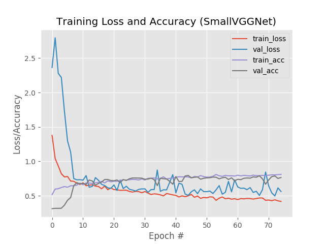
As our results demonstrate, you can see that we are achieving 76% accuracy on our Animals dataset using a Convolutional Neural Network, significantly higher than the previous accuracy of 60% using a standard fully-connected network.
We can also apply our newly trained Keras CNN to example images:
$ python predict.py --image images/panda.jpg --model output/smallvggnet.model \
	--label-bin output/smallvggnet_lb.pickle --width 64 --height 64
Using TensorFlow backend.
[INFO] loading network and label binarizer...
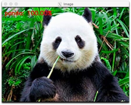
Our CNN is very confident that this a “panda”. I am too, but I just wish he would stop staring at me!
Let’s try a cute little beagle:
$ python predict.py --image images/dog.jpg --model output/smallvggnet.model \
	--label-bin output/smallvggnet_lb.pickle --width 64 --height 64
Using TensorFlow backend.
[INFO] loading network and label binarizer...
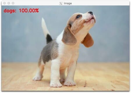
A couple beagles have been part of my family and childhood. I’m glad that this beagle picture I found online is recognized as a dog!
I could use a similar CNN to find dog photos of my beagles on my computer.
In fact, in Google Photos, if you type “dog” in the search box, pictures of dogs in your photo library will be returned — I’m pretty sure a CNN has been used for that image search engine feature. Image search engines aren’t the only use case for CNNs — I bet your mind is starting to come up with all sorts of ideas upon which to apply deep learning.
What's next? We recommend PyImageSearch University.
86+ total classes • 115+ hours hours of on-demand code walkthrough videos • Last updated: April 2026
★★★★★ 4.84 (128 Ratings) • 16,000+ Students Enrolled
I strongly believe that if you had the right teacher you could master computer vision and deep learning.
Do you think learning computer vision and deep learning has to be time-consuming, overwhelming, and complicated? Or has to involve complex mathematics and equations? Or requires a degree in computer science?
That’s not the case.
All you need to master computer vision and deep learning is for someone to explain things to you in simple, intuitive terms. And that’s exactly what I do. My mission is to change education and how complex Artificial Intelligence topics are taught.
If you're serious about learning computer vision, your next stop should be PyImageSearch University, the most comprehensive computer vision, deep learning, and OpenCV course online today. Here you’ll learn how to successfully and confidently apply computer vision to your work, research, and projects. Join me in computer vision mastery.
Inside PyImageSearch University you'll find:
- ✓ 86+ courses on essential computer vision, deep learning, and OpenCV topics
- ✓ 86 Certificates of Completion
- ✓ 115+ hours hours of on-demand video
- ✓ Brand new courses released regularly, ensuring you can keep up with state-of-the-art techniques
- ✓ Pre-configured Jupyter Notebooks in Google Colab
- ✓ Run all code examples in your web browser — works on Windows, macOS, and Linux (no dev environment configuration required!)
- ✓ Access to centralized code repos for all 540+ tutorials on PyImageSearch
- ✓ Easy one-click downloads for code, datasets, pre-trained models, etc.
- ✓ Access on mobile, laptop, desktop, etc.
Summary
In today’s tutorial, you learned how to get started with Keras, Deep Learning, and Python.
Specifically, you learned the seven key steps to working with Keras and your own custom datasets:
- How to load your data from disk
- How to create your training and testing splits
- How to define your Keras model architecture
- How to compile and prepare your Keras model
- How to train your model on your training data
- How to evaluate your model on testing data
- How to make predictions using your trained Keras model
From there you also learned how to implement a Convolutional Neural Network, enabling you to obtain higher accuracy than a standard fully-connected network.
If you have any questions regarding Keras be sure to leave a comment — I’ll do my best to answer.
And to be notified when future Keras and deep learning posts are published here on PyImageSearch, be sure to enter your email address in the form below!

Download the Source Code and FREE 17-page Resource Guide
Enter your email address below to get a .zip of the code and a FREE 17-page Resource Guide on Computer Vision, OpenCV, and Deep Learning. Inside you'll find my hand-picked tutorials, books, courses, and libraries to help you master CV and DL!
