Keras ImageDataGenerator and Data Augmentation

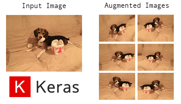
In today’s tutorial, you will learn how to use Keras’ ImageDataGenerator class to perform data augmentation. I’ll also dispel common confusions surrounding what data augmentation is, why we use data augmentation, and what it does/does not do.

Having a dataset to practice Keras ImageDataGenerator and data augmentation is beneficial in machine learning, as it allows us to artificially increase the size and diversity of our dataset, improving the ability of models to generalize.

Roboflow has free tools for each stage of the computer vision pipeline that will streamline your workflows and supercharge your productivity.

Sign up or Log in to your Roboflow account to access state of the art dataset libaries and revolutionize your computer vision pipeline.

You can start by choosing your own datasets or using our PyimageSearch’s assorted library of useful datasets.

Bring data in any of 40+ formats to Roboflow, train using any state-of-the-art model architectures, deploy across multiple platforms (API, NVIDIA, browser, iOS, etc), and connect to applications or 3rd party tools.

Knowing that I was going to write a tutorial on data augmentation, two weekends ago I decided to have some fun and purposely post a semi-trick question on my Twitter feed.

The question was simple — data augmentation does which of the following?

1. Adds more training data
2. Replaces training data
3. Does both
4. I don’t know

Here are the results:

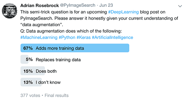
Only 5% of respondents answered this trick question “correctly” (at least if you’re using Keras’ ImageDataGenerator class).

Again, it’s a trick question so that’s not exactly a fair assessment, but here’s the deal:

While the word “augment” means to make something “greater” or “increase” something (in this case, data), the Keras ImageDataGenerator class actually works by:

1. Accepting a batch of images used for training.
2. Taking this batch and applying a series of random transformations to each image in the batch (including random rotation, resizing, shearing, etc.).
3. Replacing the original batch with the new, randomly transformed batch.
4. Training the CNN on this randomly transformed batch (i.e., the original data itself is not used for training).

That’s right — the Keras ImageDataGenerator class is not an “additive” operation. It’s not taking the original data, randomly transforming it, and then returning both the original data and transformed data.

Instead, the ImageDataGenerator accepts the original data, randomly transforms it, and returns only the new, transformed data.

But remember how I said this was a trick question?

Technically, all the answers are correct — but the only way you know if a given definition of data augmentation is correct is via the context of its application.

I’ll help you clear up some of the confusion regarding data augmentation (and give you the context you need to successfully apply it).

Inside the rest of today’s tutorial you will:

• Learn about three types of data augmentation.
• Dispel any confusion you have surrounding data augmentation.
• Learn how to apply data augmentation with Keras and the ImageDataGenerator class.

To learn more about data augmentation, including using Keras’ ImageDataGenerator class, just keep reading!

Keras ImageDataGenerator and Data Augmentation

2020-06-04 Update: This blog post is now TensorFlow 2+ compatible!

We’ll start this tutorial with a discussion of data augmentation and why we use it.

I’ll then cover the three types of data augmentation you’ll see when training deep neural networks:

1. Dataset generation and data expansion via data augmentation (less common)
2. In-place/on-the-fly data augmentation (most common)
3. Combining dataset generation and in-place augmentation

From there I’ll teach you how to apply data augmentation to your own datasets (using all three methods) using Keras’ ImageDataGenerator class.

What is data augmentation?

Data augmentation encompasses a wide range of techniques used to generate “new” training samples from the original ones by applying random jitters and perturbations (but at the same time ensuring that the class labels of the data are not changed).

Our goal when applying data augmentation is to increase the generalizability of the model.

Given that our network is constantly seeing new, slightly modified versions of the input data, the network is able to learn more robust features.

At testing time we do not apply data augmentation and simply evaluate our trained network on the unmodified testing data — in most cases, you’ll see an increase in testing accuracy, perhaps at the expense of a slight dip in training accuracy.

A simple data augmentation example

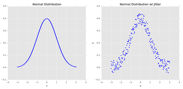
Let’s consider Figure 2 (left) of a normal distribution with zero mean and unit variance.

Training a machine learning model on this data may result in us modeling the distribution exactly — however, in real-world applications, data rarely follows such a nice, neat distribution.

Instead, to increase the generalizability of our classifier, we may first randomly jitter points along the distribution by adding some random values drawn from a random distribution (right).

Our plot still follows an approximately normal distribution, but it’s not a perfect distribution as on the left.

A model trained on this modified, augmented data is more likely to generalize to example data points not included in the training set.

Computer vision and data augmentation

In the context of computer vision, data augmentation lends itself naturally.

For example, we can obtain augmented data from the original images by applying simple geometric transforms, such as random:

1. Translations
2. Rotations
3. Changes in scale
4. Shearing
5. Horizontal (and in some cases, vertical) flips

Applying a (small) amount of the transformations to an input image will change its appearance slightly, but it does not change the class label — thereby making data augmentation a very natural, easy method to apply for computer vision tasks.

Three types of data augmentation

There are three types of data augmentation you will likely encounter when applying deep learning in the context of computer vision applications.

Exactly which definition of data augmentation is “correct” is entirely dependent on the context of your project/set of experiments.

Take the time to read this section carefully as I see many deep learning practitioners confuse what data augmentation does and does not do.

Type #1: Dataset generation and expanding an existing dataset (less common)

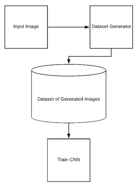
The first type of data augmentation is what I call dataset generation or dataset expansion.

As you know machine learning models, and especially neural networks, can require quite a bit of training data — but what if you don’t have very much training data in the first place?

Let’s examine the most trivial case where you only have one image and you want to apply data augmentation to create an entire dataset of images, all based on that one image.

To accomplish this task, you would:

1. Load the original input image from disk.
2. Randomly transform the original image via a series of random translations, rotations, etc.
3. Take the transformed image and write it back out to disk.
4. Repeat steps 2 and 3 a total of N times.

After performing this process you would have a directory full of randomly transformed “new” images that you could use for training, all based on that single input image.

This is, of course, an incredibly simplified example.

You more than likely have more than a single image — you probably have 10s or 100s of images and now your goal is to turn that smaller set into 1000s of images for training.

In those situations, dataset expansion and dataset generation may be worth exploring.

But there’s a problem with this approach — we haven’t exactly increased the ability of our model to generalize.

Yes, we have increased our training data by generating additional examples, but all of these examples are based on a super small dataset.

Keep in mind that our neural network is only as good as the data it was trained on.

We cannot expect to train a NN on a small amount of data and then expect it to generalize to data it was never trained on and has never seen before.

If you find yourself seriously considering dataset generation and dataset expansion, you should take a step back and instead invest your time gathering additional data or looking into methods of behavioral cloning (and then applying the type of data augmentation covered in the “Combining dataset generation and in-place augmentation” section below).

Type #2: In-place/on-the-fly data augmentation (most common)

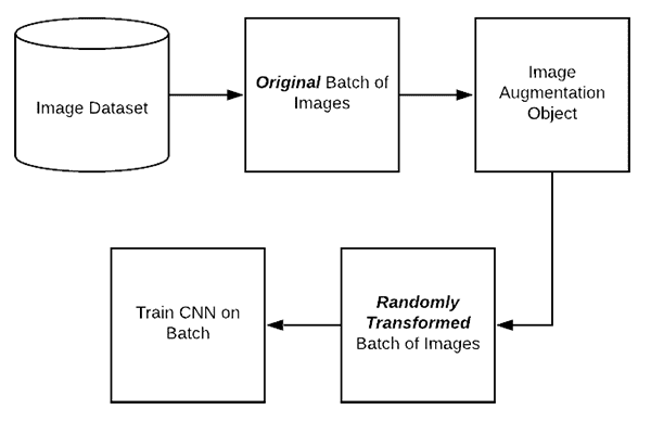
The second type of data augmentation is called in-place data augmentation or on-the-fly data augmentation. This type of data augmentation is what Keras’ ImageDataGenerator class implements.

Using this type of data augmentation we want to ensure that our network, when trained, sees new variations of our data at each and every epoch.

Figure 5 demonstrates the process of applying in-place data augmentation:

1. Step #1: An input batch of images is presented to the ImageDataGenerator .
2. Step #2: The ImageDataGenerator transforms each image in the batch by a series of random translations, rotations, etc.
3. Step #3: The randomly transformed batch is then returned to the calling function.

There are two important points that I want to draw your attention to:

1. The ImageDataGenerator is not returning both the original data and the transformed data — the class only returns the randomly transformed data.
2. We call this “in-place” and “on-the-fly” data augmentation because this augmentation is done at training time (i.e., we are not generating these examples ahead of time/prior to training).

When our model is being trained, we can think of our ImageDataGenerator class as “intercepting” the original data, randomly transforming it, and then returning it to the neural network for training, all the while the NN has no idea the data was modified!

I’ve written previous tutorials on the PyImageSearch blog where readers think that Keras’ ImageDateGenerator class is an “additive operation”, similar to the following (incorrect) figure:

In the above illustration the ImageDataGenerator accepts an input batch of images, randomly transforms the batch, and then returns both the original batch and modified data — again, this is not what the Keras ImageDataGenerator does. Instead, the ImageDataGenerator class will return just the randomly transformed data.

When I explain this concept to readers the next question is often:

But Adrian, what about the original training data? Why is it not used? Isn’t the original training data still useful for training?

Keep in mind that the entire point of the data augmentation technique described in this section is to ensure that the network sees “new” images that it has never “seen” before at each and every epoch.

If we included the original training data along with the augmented data in each batch, then the network would “see” the original training data multiple times, effectively defeating the purpose. Secondly, recall that the overall goal of data augmentation is to increase the generalizability of the model.

To accomplish this goal we “replace” the training data with randomly transformed, augmented data.

In practice, this leads to a model that performs better on our validation/testing data but perhaps performs slightly worse on our training data (to due to the variations in data caused by the random transforms).

You’ll learn how to use the Keras ImageDataGenerator class later in this tutorial.

Type #3: Combining dataset generation and in-place augmentation

The final type of data augmentation seeks to combine both dataset generation and in-place augmentation — you may see this type of data augmentation when performing behavioral cloning.

A great example of behavioral cloning can be seen in self-driving car applications.

Creating self-driving car datasets can be extremely time consuming and expensive — a way around the issue is to instead use video games and car driving simulators.

Video game graphics have become so life-like that it’s now possible to use them as training data.

Therefore, instead of driving an actual vehicle, you can instead:

• Play a video game
• Write a program to play a video game
• Use the underlying rendering engine of the video game

…all to generate actual data that can be used for training.

Once you have your training data you can go back and apply Type #2 data augmentation (i.e., in-place/on-the-fly data augmentation) to the data you gathered via your simulation.

Configuring your development environment

To configure your system for this tutorial, I first recommend following either of these tutorials:

• How to install TensorFlow 2.0 on Ubuntu
• How to install TensorFlow 2.0 on macOS

Either tutorial will help you configure you system with all the necessary software for this blog post in a convenient Python virtual environment.

Please note that PyImageSearch does not recommend or support Windows for CV/DL projects.

Project structure

Before we dive into the code let’s first review our directory structure for the project:

$ tree --dirsfirst --filelimit 10
.
├── dogs_vs_cats_small
│   ├── cats [1000 entries]
│   └── dogs [1000 entries]
├── generated_dataset
│   ├── cats [100 entries]
│   └── dogs [100 entries]
├── pyimagesearch
│   ├── __init__.py
│   └── resnet.py
├── cat.jpg
├── dog.jpg
├── plot_dogs_vs_cats_no_aug.png
├── plot_dogs_vs_cats_with_aug.png
├── plot_generated_dataset.png
├── train.py
└── generate_images.py

7 directories, 9 files

First, there are two dataset directories which are not to be confused:

• dogs_vs_cats_small/ : A subset of the popular Kaggle Dogs vs. Cats competition dataset. In my curated subset, only 2,000 images (1,000 per class) are present (as opposed to the 25,000 images for the challenge).
• generated_dataset/ : We’ll create this generated dataset using the cat.jpg and dog.jpg images which are in the parent directory. We’ll utilize data augmentation Type #1 to generate this dataset automatically and fill this directory with images.

Next, we have our pyimagesearch module which contains our implementation of the ResNet CNN classifier.

Today, we’ll review two Python scripts:

• train.py : Used to train models for both Type #1 and Type #2 (and optionally Type #3 if the user so wishes) data augmentation techniques. We’ll perform three training experiments resulting in each of the three plot*.png files in the project folder.
• generate_images.py : Used to generate a dataset from a single image using Type #1.

Let’s begin.

Implementing our training script

In the remainder of this tutorial we’ll be performing three experiments:

1. Experiment #1: Generate a dataset via dataset expansion and train a CNN on it.
2. Experiment #2: Use a subset of the Kaggle Dogs vs. Cats dataset and train a CNN without data augmentation.
3. Experiment #3: Repeat the second experiment, but this time with data augmentation.

All of these experiments will be accomplished using the same Python script.

Open up the train.py script and let’s get started:

# set the matplotlib backend so figures can be saved in the background
import matplotlib
matplotlib.use("Agg")

# import the necessary packages
from pyimagesearch.resnet import ResNet
from sklearn.preprocessing import LabelEncoder
from sklearn.model_selection import train_test_split
from sklearn.metrics import classification_report
from tensorflow.keras.preprocessing.image import ImageDataGenerator
from tensorflow.keras.optimizers import SGD
from tensorflow.keras.utils import to_categorical
from imutils import paths
import matplotlib.pyplot as plt
import numpy as np
import argparse
import cv2
import os

On Lines 2-18 our necessary packages are imported. Line 10 is our ImageDataGenerator import from the Keras library — a class for data augmentation.

Let’s go ahead and parse our command line arguments:

# construct the argument parser and parse the arguments
ap = argparse.ArgumentParser()
ap.add_argument("-d", "--dataset", required=True,
	help="path to input dataset")
ap.add_argument("-a", "--augment", type=int, default=-1,
	help="whether or not 'on the fly' data augmentation should be used")
ap.add_argument("-p", "--plot", type=str, default="plot.png",
	help="path to output loss/accuracy plot")
args = vars(ap.parse_args())

Our script accepts three command line arguments via the terminal:

• --dataset : The path to the input dataset.
• --augment : Whether “on-the-fly” data augmentation should be used (refer to type #2 above). By default, this method is not performed.
• --plot : The path to the output training history plot.

Let’s proceed to initialize hyperparameters and load our image data:

# initialize the initial learning rate, batch size, and number of
# epochs to train for
INIT_LR = 1e-1
BS = 8
EPOCHS = 50

# grab the list of images in our dataset directory, then initialize
# the list of data (i.e., images) and class images
print("[INFO] loading images...")
imagePaths = list(paths.list_images(args["dataset"]))
data = []
labels = []

# loop over the image paths
for imagePath in imagePaths:
	# extract the class label from the filename, load the image, and
	# resize it to be a fixed 64x64 pixels, ignoring aspect ratio
	label = imagePath.split(os.path.sep)[-2]
	image = cv2.imread(imagePath)
	image = cv2.resize(image, (64, 64))

	# update the data and labels lists, respectively
	data.append(image)
	labels.append(label)

Training hyperparameters, including initial learning rate, batch size, and number of epochs to train for, are initialized on Lines 32-34.

From there Lines 39-53 grab imagePaths , load images, and populate our data and labels lists. The only image preprocessing we perform at this point is to resize each image to 64×64px.

Next, let’s finish preprocessing, encode our labels, and partition our data:

# convert the data into a NumPy array, then preprocess it by scaling
# all pixel intensities to the range [0, 1]
data = np.array(data, dtype="float") / 255.0

# encode the labels (which are currently strings) as integers and then
# one-hot encode them
le = LabelEncoder()
labels = le.fit_transform(labels)
labels = to_categorical(labels, 2)

# partition the data into training and testing splits using 75% of
# the data for training and the remaining 25% for testing
(trainX, testX, trainY, testY) = train_test_split(data, labels,
	test_size=0.25, random_state=42)

On Line 57, we convert data to a NumPy array as well as scale all pixel intensities to the range [0, 1]. This completes our preprocessing.

From there we perform “one-hot encoding” of our labels (Lines 61-63). This method of encoding our labels results in an array that may look like this:

array([[0., 1.],
       [0., 1.],
       [0., 1.],
       [1., 0.],
       [1., 0.],
       [0., 1.],
       [0., 1.]], dtype=float32)

For this sample of data, there are two cats ([1., 0.] ) and five dogs ([0., 1] ) where the label corresponding to the image is marked as “hot”.

From there we partition our data into training and testing splits marking 75% of our data for training and the remaining 25% for testing (Lines 67 and 68).

Now, we are ready to initialize our data augmentation object:

# initialize an our data augmenter as an "empty" image data generator
aug = ImageDataGenerator()

Line 71 initializes our empty data augmentation object (i.e., no augmentation will be performed). This is the default operation of this script.

Let’s check if we’re going to override the default with the --augment command line argument:

# check to see if we are applying "on the fly" data augmentation, and
# if so, re-instantiate the object
if args["augment"] > 0:
	print("[INFO] performing 'on the fly' data augmentation")
	aug = ImageDataGenerator(
		rotation_range=20,
		zoom_range=0.15,
		width_shift_range=0.2,
		height_shift_range=0.2,
		shear_range=0.15,
		horizontal_flip=True,
		fill_mode="nearest")

Line 75 checks to see if we are performing data augmentation. If so, we re-initialize the data augmentation object with random transformation parameters (Lines 77-84). As the parameters indicate, random rotations, zooms, shifts, shears, and flips will be performed during in-place/on-the-fly data augmentation.

Let’s compile and train our model:

# initialize the optimizer and model
print("[INFO] compiling model...")
opt = SGD(lr=INIT_LR, momentum=0.9, decay=INIT_LR / EPOCHS)
model = ResNet.build(64, 64, 3, 2, (2, 3, 4),
	(32, 64, 128, 256), reg=0.0001)
model.compile(loss="binary_crossentropy", optimizer=opt,
	metrics=["accuracy"])

# train the network
print("[INFO] training network for {} epochs...".format(EPOCHS))
H = model.fit(
	x=aug.flow(trainX, trainY, batch_size=BS),
	validation_data=(testX, testY),
	steps_per_epoch=len(trainX) // BS,
	epochs=EPOCHS)

2020-06-04 Update: Formerly, TensorFlow/Keras required use of a method called .fit_generator in order to accomplish data augmentation. Now, the .fit method can handle data augmentation as well, making for more-consistent code. This also applies to the migration from .predict_generator to .predict. Be sure to check out my other article fit and fit_generator after you’re done reading this tutorial.

Lines 88-92 construct our ResNet model using Stochastic Gradient Descent optimization and learning rate decay. We use "binary_crossentropy" loss for this 2-class problem. If you have more than two classes, be sure to use "categorial_crossentropy" .

Lines 96-100 then train our model. The aug object handles data augmentation in batches (although be sure to recall that the aug object will only perform data augmentation if the --augment command line argument was set).

Finally, we’ll evaluate our model, print statistics, and generate a training history plot:

# evaluate the network
print("[INFO] evaluating network...")
predictions = model.predict(x=testX.astype("float32"), batch_size=BS)
print(classification_report(testY.argmax(axis=1),
	predictions.argmax(axis=1), target_names=le.classes_))

# plot the training loss and accuracy
N = np.arange(0, EPOCHS)
plt.style.use("ggplot")
plt.figure()
plt.plot(N, H.history["loss"], label="train_loss")
plt.plot(N, H.history["val_loss"], label="val_loss")
plt.plot(N, H.history["accuracy"], label="train_acc")
plt.plot(N, H.history["val_accuracy"], label="val_acc")
plt.title("Training Loss and Accuracy on Dataset")
plt.xlabel("Epoch #")
plt.ylabel("Loss/Accuracy")
plt.legend(loc="lower left")
plt.savefig(args["plot"])

2020-06-04 Update: In order for this plotting snippet to be TensorFlow 2+ compatible the H.history dictionary keys are updated to fully spell out “accuracy” sans “acc” (i.e., H.history["val_accuracy"] and H.history["accuracy"]). It is semi-confusing that “val” is not spelled out as “validation”; we have to learn to love and live with the API and always remember that it is a work in progress that many developers around the world contribute to.

Line 104 makes predictions on the test set for evaluation purposes. A classification report is printed via Lines 105 and 106.

From there, Lines 109-120 generate and save an accuracy/loss training plot.

Generating a dataset/dataset expansion with data augmentation and Keras

In our first experiment, we will perform dataset expansion via data augmentation with Keras.

Our dataset will contain 2 classes and initially, the dataset will trivially contain only 1 image per class:

• Cat: 1 image
• Dog: 1 image

We’ll utilize Type #1 data augmentation (see the “Type #1: Dataset generation and expanding an existing dataset” section above) to generate a new dataset with 100 images per class:

• Cat: 100 images
• Dog: 100 images

Again, this meant to be an example — in a real-world application you would have 100s of example images, but we’re keeping it simple here so you can learn the concept.

Generating the example dataset

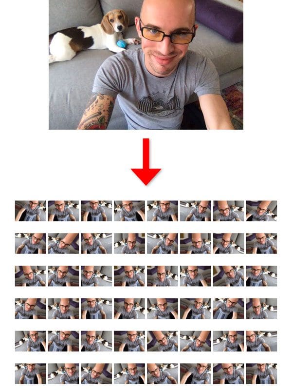
Before we can train our CNN we first need to generate an example dataset.

From our “Project Structure” section above you know that we have two example images in our root directory: cat.jpg and dog.jpg. We will use these example images to generate 100 new training images per class (200 images in total).

To see how we can use data augmentation to generate new examples, open up the generate_images.py file and follow along:

# import the necessary packages
from tensorflow.keras.preprocessing.image import ImageDataGenerator
from tensorflow.keras.preprocessing.image import img_to_array
from tensorflow.keras.preprocessing.image import load_img
import numpy as np
import argparse

# construct the argument parser and parse the arguments
ap = argparse.ArgumentParser()
ap.add_argument("-i", "--image", required=True,
	help="path to the input image")
ap.add_argument("-o", "--output", required=True,
	help="path to output directory to store augmentation examples")
ap.add_argument("-t", "--total", type=int, default=100,
	help="# of training samples to generate")
args = vars(ap.parse_args())

Lines 2-6 import our necessary packages. Our ImageDataGenerator is imported on Line 2 and will handle our data augmentation with Keras.

From there, we’ll parse three command line arguments:

• --image : The path to the input image. We’ll generate additional random, mutated versions of this image.
• --output : The path to the output directory to store the data augmentation examples.
• --total : The number of sample images to generate.

Let’s go ahead and load our image and initialize our data augmentation object:

# load the input image, convert it to a NumPy array, and then
# reshape it to have an extra dimension
print("[INFO] loading example image...")
image = load_img(args["image"])
image = img_to_array(image)
image = np.expand_dims(image, axis=0)

# construct the image generator for data augmentation then
# initialize the total number of images generated thus far
aug = ImageDataGenerator(
	rotation_range=30,
	zoom_range=0.15,
	width_shift_range=0.2,
	height_shift_range=0.2,
	shear_range=0.15,
	horizontal_flip=True,
	fill_mode="nearest")
total = 0

Our image is loaded and prepared for data augmentation via Lines 21-23. Image loading and processing is handled via Keras functionality (i.e. we aren’t using OpenCV).

From there, we initialize the ImageDataGenerator object. This object will facilitate performing random rotations, zooms, shifts, shears, and flips on our input image.

Next, we’ll construct a Python generator and put it to work until all of our images have been produced:

# construct the actual Python generator
print("[INFO] generating images...")
imageGen = aug.flow(image, batch_size=1, save_to_dir=args["output"],
	save_prefix="image", save_format="jpg")

# loop over examples from our image data augmentation generator
for image in imageGen:
	# increment our counter
	total += 1

	# if we have reached the specified number of examples, break
	# from the loop
	if total == args["total"]:
		break

We will use the imageGen to randomly transform the input image (Lines 39 and 40). This generator saves images as .jpg files to the specified output directory contained within args["output"] .

Finally, we’ll loop over examples from our image data generator and count them until we’ve reached the required total number of images.

To run the generate_examples.py script make sure you have used the “Downloads” section of the tutorial to download the source code and example images.

From there open up a terminal and execute the following command:

$ python generate_images.py --image cat.jpg --output generated_dataset/cats
[INFO] loading example image...
[INFO] generating images...

Check the output of the generated_dataset/cats directory you will now see 100 images:

$ ls generated_dataset/cats/*.jpg | wc -l
     100

Let’s do the same now for the “dogs” class:

$ python generate_images.py --image dog.jpg --output generated_dataset/dogs
[INFO] loading example image...
[INFO] generating images...

And now check for the dog images:

$ ls generated_dataset/dogs/*.jpg | wc -l
     100

A visualization of the dataset generation via data augmentation can be seen in Figure 6 at the top of this section — notice how we have accepted a single input image (of me — not of a dog or cat) and then created 100 new training examples (48 of which are visualized) from that single image.

Experiment #1: Dataset generation results

We are now ready to perform our first experiment:

$ python train.py --dataset generated_dataset --plot plot_generated_dataset.png
[INFO] loading images...
[INFO] compiling model...
[INFO] training network for 50 epochs...
Epoch 1/50
18/18 [==============================] - 1s 60ms/step - loss: 0.3191 - accuracy: 0.9220 - val_loss: 0.1986 - val_accuracy: 1.0000
Epoch 2/50
18/18 [==============================] - 0s 9ms/step - loss: 0.2276 - accuracy: 0.9858 - val_loss: 0.2044 - val_accuracy: 1.0000
Epoch 3/50
18/18 [==============================] - 0s 8ms/step - loss: 0.2839 - accuracy: 0.9574 - val_loss: 0.2046 - val_accuracy: 1.0000
...
Epoch 48/50
18/18 [==============================] - 0s 9ms/step - loss: 0.1770 - accuracy: 1.0000 - val_loss: 0.1768 - val_accuracy: 1.0000
Epoch 49/50
18/18 [==============================] - 0s 9ms/step - loss: 0.1767 - accuracy: 1.0000 - val_loss: 0.1763 - val_accuracy: 1.0000
Epoch 50/50
18/18 [==============================] - 0s 8ms/step - loss: 0.1767 - accuracy: 1.0000 - val_loss: 0.1758 - val_accuracy: 1.0000
[INFO] evaluating network...
              precision    recall  f1-score   support

        cats       1.00      1.00      1.00        25
        dogs       1.00      1.00      1.00        25

    accuracy                           1.00        50
   macro avg       1.00      1.00      1.00        50
weighted avg       1.00      1.00      1.00        50

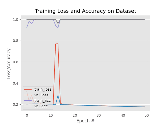
Our results show that we were able to obtain 100% accuracy with little effort.

Of course, this is a trivial, contrived example. In practice, you would not be taking only a single image and then building a dataset of 100s or 1000s of images via data augmentation. Instead, you would have a dataset of 100s of images and then you would apply dataset generation to that dataset — but again, the point of this section was to demonstrate on a simple example so you could understand the process.

Training a network with in-place data augmentation

The more popular form of (image-based) data augmentation is called in-place data augmentation (see the “Type #2: In-place/on-the-fly data augmentation” section of this post for more details).

When performing in-place augmentation our Keras ImageDataGenerator will:

1. Accept a batch of input images.
2. Randomly transform the input batch.
3. Return the transformed batch to the network for training.

We’ll explore how data augmentation can reduce overfitting and increase the ability of our model to generalize via two experiments.

To accomplish this task we’ll be using a subset of the Kaggle Dogs vs. Cats dataset:

• Cats: 1,000 images
• Dogs: 1,000 images

We’ll then train a variation of ResNet, from scratch, on this dataset with and without data augmentation.

Experiment #2: Obtaining a baseline (no data augmentation)

In our first experiment we’ll perform no data augmentation:

$ python train.py --dataset dogs_vs_cats_small --plot plot_dogs_vs_cats_no_aug.png
[INFO] loading images...
[INFO] compiling model...
[INFO] training network for 50 epochs...
Epoch 1/50
187/187 [==============================] - 3s 13ms/step - loss: 1.0743 - accuracy: 0.5134 - val_loss: 0.9116 - val_accuracy: 0.5440
Epoch 2/50
187/187 [==============================] - 2s 9ms/step - loss: 0.9149 - accuracy: 0.5349 - val_loss: 0.9055 - val_accuracy: 0.4940
Epoch 3/50
187/187 [==============================] - 2s 9ms/step - loss: 0.9065 - accuracy: 0.5409 - val_loss: 0.8990 - val_accuracy: 0.5360
...
Epoch 48/50
187/187 [==============================] - 2s 9ms/step - loss: 0.2796 - accuracy: 0.9564 - val_loss: 1.4528 - val_accuracy: 0.6500
Epoch 49/50
187/187 [==============================] - 2s 10ms/step - loss: 0.2806 - accuracy: 0.9578 - val_loss: 1.4485 - val_accuracy: 0.6260
Epoch 50/50
187/187 [==============================] - 2s 9ms/step - loss: 0.2371 - accuracy: 0.9739 - val_loss: 1.5061 - val_accuracy: 0.6380
[INFO] evaluating network...
              precision    recall  f1-score   support

        cats       0.61      0.70      0.65       243
        dogs       0.67      0.58      0.62       257

    accuracy                           0.64       500
   macro avg       0.64      0.64      0.64       500
weighted avg       0.64      0.64      0.64       500

Looking at the raw classification report you’ll see that we’re obtaining 64% accuracy — but there’s a problem!

Take a look at the plot associated with our training:

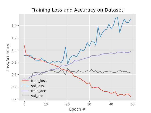
There is dramatic overfitting occurring — at approximately epoch 15 we see our validation loss start to rise while training loss continues to fall. By epoch 20 the rise in validation loss is especially pronounced.

This type of behavior is indicative of overfitting.

The solution is to (1) reduce model capacity, and/or (2) perform regularization.

Experiment #3: Improving our results (with data augmentation)

Let’s now investigate how data augmentation can act as a form of regularization:

[INFO] loading images...
[INFO] performing 'on the fly' data augmentation
[INFO] compiling model...
[INFO] training network for 50 epochs...
Epoch 1/50
187/187 [==============================] - 3s 14ms/step - loss: 1.1307 - accuracy: 0.4940 - val_loss: 0.9002 - val_accuracy: 0.4860
Epoch 2/50
187/187 [==============================] - 2s 8ms/step - loss: 0.9172 - accuracy: 0.5067 - val_loss: 0.8952 - val_accuracy: 0.6000
Epoch 3/50
187/187 [==============================] - 2s 8ms/step - loss: 0.8930 - accuracy: 0.5074 - val_loss: 0.8801 - val_accuracy: 0.5040
...
Epoch 48/50
187/187 [==============================] - 2s 8ms/step - loss: 0.7194 - accuracy: 0.6937 - val_loss: 0.7296 - val_accuracy: 0.7060
Epoch 49/50
187/187 [==============================] - 2s 8ms/step - loss: 0.7071 - accuracy: 0.6971 - val_loss: 0.7690 - val_accuracy: 0.6980
Epoch 50/50
187/187 [==============================] - 2s 9ms/step - loss: 0.6901 - accuracy: 0.7091 - val_loss: 0.7957 - val_accuracy: 0.6840
[INFO] evaluating network...
              precision    recall  f1-score   support

        cats       0.72      0.56      0.63       243
        dogs       0.66      0.80      0.72       257

    accuracy                           0.68       500
   macro avg       0.69      0.68      0.68       500
weighted avg       0.69      0.68      0.68       500

We’re now up to 69% accuracy, an increase from our previous 64% accuracy.

But more importantly, we are no longer overfitting:

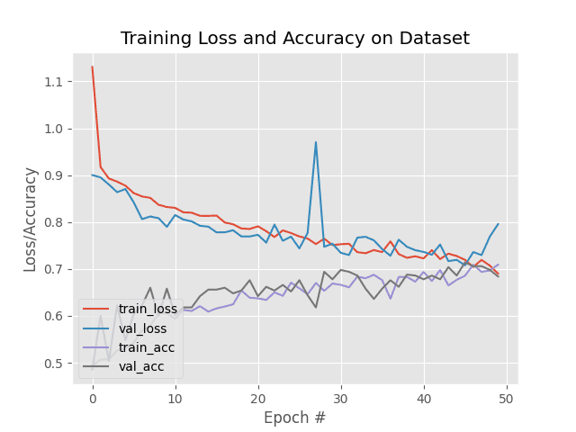
Note how validation and training loss are falling together with little divergence. Similarly, classification accuracy for both the training and validation splits are growing together as well.

By using data augmentation we were able to combat overfitting!

In nearly all situations, unless you have very good reason not to, you should be performing data augmentation when training your own neural networks.

Summary

In this tutorial, you learned about data augmentation and how to apply data augmentation via Keras’ ImageDataGenerator class.

You also learned about three types of data augmentation, including:

1. Dataset generation and data expansion via data augmentation (less common).
2. In-place/on-the-fly data augmentation (most common).
3. Combining the dataset generator and in-place augmentation.

By default, Keras’ ImageDataGenerator class performs in-place/on-the-fly data augmentation, meaning that the class:

1. Accepts a batch of images used for training.
2. Takes this batch and applies a series of random transformations to each image in the batch.
3. Replaces the original batch with the new, randomly transformed batch
4. 4. Trains the CNN on this randomly transformed batch (i.e., the original data itself is not used for training).

All that said, we actually can take the ImageDataGenerator class and use it for dataset generation/expansion as well — we just need to use it to generate our dataset before training.

The final method of data augmentation, combining both in-place and dataset expansion, is rarely used. In those situations, you likely have a small dataset, need to generate additional examples via data augmentation, and then have an additional augmentation/preprocessing at training time.

We wrapped up the guide by performing a number of experiments with data augmentation, noting that data augmentation is a form of regularization, enabling our network to generalize better to our testing/validation set.

This claim of data augmentation as regularization was verified in our experiments when we found that:

1. Not applying data augmentation at training caused overfitting
2. While apply data augmentation allowed for smooth training, no overfitting, and higher accuracy/lower loss

You should apply data augmentation in all of your experiments unless you have a very good reason not to.

To learn more about data augmentation, including my best practices, tips, and suggestions, be sure to take a look at my book, Deep Learning for Computer Vision with Python.

I hope you enjoyed today’s tutorial!

To download the source code to this post (and receive email updates when future tutorials are published here on PyImageSearch), just enter your email address in the form below!