LeNet – Convolutional Neural Network in Python

In today’s blog post, we are going to implement our first Convolutional Neural Network (CNN) — LeNet — using Python and the Keras deep learning package.

The LeNet architecture was first introduced by LeCun et al. in their 1998 paper, Gradient-Based Learning Applied to Document Recognition. As the name of the paper suggests, the authors’ implementation of LeNet was used primarily for OCR and character recognition in documents.

The LeNet architecture is straightforward and small, (in terms of memory footprint), making it perfect for teaching the basics of CNNs — it can even run on the CPU (if your system does not have a suitable GPU), making it a great “first CNN”.

However, if you do have GPU support and can access your GPU via Keras, you will enjoy extremely fast training times (in the order of 3-10 seconds per epoch, depending on your GPU).

In the remainder of this post, I’ll be demonstrating how to implement the LeNet Convolutional Neural Network architecture using Python and Keras.

From there, I’ll show you how to train LeNet on the MNIST dataset for digit recognition.

To learn how to train your first Convolutional Neural Network, keep reading.

LeNet – Convolutional Neural Network in Python

This tutorial will be primarily code oriented and meant to help you get your feet wet with Deep Learning and Convolutional Neural Networks. Because of this intention, I am not going to spend a lot of time discussing activation functions, pooling layers, or dense/fully-connected layers — there will be plenty of tutorials on the PyImageSearch blog in the future that will cover each of these layer types/concepts in lots of detail.

Again, this tutorial is meant to be your first end-to-end example where you get to train a real-life CNN (and see it in action). We’ll get to the gory details of activation functions, pooling layers, and fully-connected layers later in this series of posts (although you should already know the basics of how convolution operations work); but in the meantime, simply follow along, enjoy the lesson, and learn how to implement your first Convolutional Neural Network with Python and Keras.

The MNIST dataset

You’ve likely already seen the MNIST dataset before, either here on the PyImageSearch blog, or elsewhere in your studies. In either case, I’ll go ahead and quickly review the dataset to ensure you know exactly what data we’re working with.

The MNIST dataset is arguably the most well-studied, most understood dataset in the computer vision and machine learning literature, making it an excellent “first dataset” to use on your deep learning journey.

Note: As we’ll find out, it’s also quite easy to get > 98% classification accuracy on this dataset with minimal training time, even on the CPU.

The goal of this dataset is to classify the handwritten digits 0-9. We’re given a total of 70,000 images, with (normally) 60,000 images used for training and 10,000 used for evaluation; however, we’re free to split this data as we see fit. Common splits include the standard 60,000/10,000, 75%/25%, and 66.6%/33.3%. I’ll be using 2/3 of the data for training and 1/3 of the data for testing later in the blog post.

Each digit is represented as a 28 x 28 grayscale image (examples from the MNIST dataset can be seen in the figure above). These grayscale pixel intensities are unsigned integers, with the values of the pixels falling in the range [0, 255]. All digits are placed on a black background with a light foreground (i.e., the digit itself) being white and various shades of gray.

It’s worth noting that many libraries (such as scikit-learn) have built-in helper methods to download the MNIST dataset, cache it locally to disk, and then load it. These helper methods normally represent each image as a 784-d vector.

Where does the number 784 come from?

Simple. It’s just the flattened 28 x 28 = 784 image.

To recover our original image from the 784-d vector, we simply reshape the array into a 28 x 28 image.

In the context of this blog post, our goal is to train LeNet such that we maximize accuracy on our testing set.

The LeNet architecture

The LeNet architecture is an excellent “first architecture” for Convolutional Neural Networks (especially when trained on the MNIST dataset, an image dataset for handwritten digit recognition).

LeNet is small and easy to understand — yet large enough to provide interesting results. Furthermore, the combination of LeNet + MNIST is able to run on the CPU, making it easy for beginners to take their first step in Deep Learning and Convolutional Neural Networks.

In many ways, LeNet + MNIST is the “Hello, World” equivalent of Deep Learning for image classification.

The LeNet architecture consists of the following layers:

INPUT => CONV => RELU => POOL => CONV => RELU => POOL => FC => RELU => FC

Instead of explaining the number of convolution filters per layer, the size of the filters themselves, and the number of fully-connected nodes right now, I’m going to save this discussion until our “Implementing LeNet with Python and Keras” section of the blog post where the source code will serve as an aid in the explantation.

In the meantime, let’s took at our project structure — a structure that we are going to reuse many times in future PyImageSearch blog posts.

Note: The original LeNet architecture used TANH activation functions rather than RELU . The reason we use RELU here is because it tends to give much better classification accuracy due to a number of nice, desirable properties (which I’ll discuss in a future blog post). If you run into any other discussions on LeNet, you might see that they use TANH instead — again, just something to keep in mind.

Our CNN project structure

Before we dive into any code, let’s first review our project structure:

|--- output
|--- pyimagesearch
|    |--- __init__.py
|    |--- cnn
|    |    |--- __init__.py
|    |    |--- networks
|    |    |    |--- __init__.py
|    |    |    |--- lenet.py
|--- lenet_mnist.py

To keep our code organized, we’ll define a package named pyimagesearch . And within the pyimagesearch module, we’ll create a cnn sub-module — this is where we’ll store our Convolutional Neural Network implementations, along with any helper utilities related to CNNs.

Taking a look inside cnn , you’ll see the networks sub-module: this is where the network implementations themselves will be stored. As the name suggests, the lenet.py file will define a class named LeNet , which is our actual LeNet implementation in Python + Keras.

The lenet_mnist.py script will be our driver program used to instantiate the LeNet network architecture, train the model (or load the model, if our network is pre-trained), and then evaluate the network performance on the MNIST dataset.

Finally, the output directory will store our LeNet model after it has been trained, allowing us to classify digits in subsequent calls to lenet_mnist.py without having to re-train the network.

I personally have been using this project structure (or a project structure very similar to it) over the past year. I’ve found it well organized and easy to extend — this will become more evident in future blog posts as we add to this library with more network architectures and helper functions.

Implementing LeNet with Python and Keras

To start, I am going to assume that you already have Keras, scikit-learn, and OpenCV installed on your system (and optionally, have GPU-support enabled). If you do not, please refer to this blog post to help you get your system configured properly.

Otherwise, open up the lenet.py file and insert the following code:

# import the necessary packages
from keras.models import Sequential
from keras.layers.convolutional import Conv2D
from keras.layers.convolutional import MaxPooling2D
from keras.layers.core import Activation
from keras.layers.core import Flatten
from keras.layers.core import Dense
from keras import backend as K

class LeNet:
	@staticmethod
	def build(numChannels, imgRows, imgCols, numClasses,
		activation="relu", weightsPath=None):
		# initialize the model
		model = Sequential()
		inputShape = (imgRows, imgCols, numChannels)

		# if we are using "channels first", update the input shape
		if K.image_data_format() == "channels_first":
			inputShape = (numChannels, imgRows, imgCols)

Lines 2-8 handle importing the required functions/classes from the keras library.

The LeNet class is defined on Line 10, followed by the build method on Line 12. Whenever I define a new network architecture, I always place it in its own class (mainly for namespace and organization purposes) — followed by creating a static build function.

The build method, as the name suggests, takes any supplied parameters, which at a bare minimum include:

• The width of our input images.
• The height of our input images.
• The depth (i.e., number of channels) of our input images.
• And the number of classes (i.e., unique number of class labels) in our dataset.

I also normally include a weightsPath which can be used to load a pre-trained model. Given these parameters, the build function is responsible for constructing the network architecture.

Speaking of building the LeNet architecture, Line 15 instantiates a Sequential class which we’ll use to construct the network.

Then, we handle whether we’re working with “channels last” or “channels first” tensors on Lines 16-20. Tensorflow’s default is “channels last”.

Now that the model has been initialized, we can start adding layers to it:

		# define the first set of CONV => ACTIVATION => POOL layers
		model.add(Conv2D(20, 5, padding="same",
			input_shape=inputShape))
		model.add(Activation(activation))
		model.add(MaxPooling2D(pool_size=(2, 2), strides=(2, 2)))

On Lines 23-26 we create our first set of CONV => RELU => POOL layer sets.

Our CONV layer will learn 20 convolution filters, where each filter is of size 5 x 5. The input dimensions of this value are the same width, height, and depth as our input images — in this case, the MNIST dataset, so we’ll have 28 x 28 inputs with a single channel for depth (grayscale).

We’ll then apply the ReLU activation function followed by 2 x 2 max-pooling in both the x and y direction with a stride of 2 (imagine a 2 x 2 sliding window that “slides” across the activation volume, taking the max operation of each region, while taking a step of 2 pixels in both the horizontal and vertical direction).

Note: This tutorial is primarily code based and is meant to be your first exposure to implementing a Convolutional Neural Network — I’ll be going into lots more detail regarding convolutional layers, activation functions, and max-pooling layers in future blog posts. In the meantime, simply try to follow along with the code.

We are now ready to apply our second set of CONV => RELU => POOL layers:

		# define the second set of CONV => ACTIVATION => POOL layers
		model.add(Conv2D(50, 5, padding="same"))
		model.add(Activation(activation))
		model.add(MaxPooling2D(pool_size=(2, 2), strides=(2, 2)))

This time we’ll be learning 50 convolutional filters rather than the 20 convolutional filters as in the previous layer set.

It’s common to see the number of CONV filters learned increase in deeper layers of the network.

Next, we come to the fully-connected layers (often called “dense” layers) of the LeNet architecture:

		# define the first FC => ACTIVATION layers
		model.add(Flatten())
		model.add(Dense(500))
		model.add(Activation(activation))

		# define the second FC layer
		model.add(Dense(numClasses))

		# lastly, define the soft-max classifier
		model.add(Activation("softmax"))

On Line 34 we take the output of the preceding MaxPooling2D layer and flatten it into a single vector, allowing us to apply dense/fully-connected layers. If you have any prior experience with neural networks, then you’ll know that a dense/fully-connected layer is a “standard” type of layer in a network, where every node in the preceding layer connects to every node in the next layer (hence the term, “fully-connected”).

Our fully-connected layer will contain 500 units (Line 35) which we pass through another nonlinear ReLU activation.

Line 39 is very important, although it’s easy to overlook — this line defines another Dense class, but accepts a variable (i.e., not hardcoded) size. This size is the number of class labels represented by the classes variable. In the case of the MNIST dataset, we have 10 classes (one for each of the ten digits we are trying to learn to recognize).

Finally, we apply a softmax classifier (multinomial logistic regression) that will return a list of probabilities, one for each of the 10 class labels (Line 42). The class label with the largest probability will be chosen as the final classification from the network.

Our last code block handles loading a pre-existing weightsPath (if such a file exists) and returning the constructed model to the calling function:

		# if a weights path is supplied (inicating that the model was
		# pre-trained), then load the weights
		if weightsPath is not None:
			model.load_weights(weightsPath)

		# return the constructed network architecture
		return model

Creating the LeNet driver script

Now that we have implemented the LeNet Convolutional Neural Network architecture using Python + Keras, it’s time to define the lenet_mnist.py driver script which will handle:

1. Loading the MNIST dataset.
2. Partitioning MNIST into training and testing splits.
3. Loading and compiling the LeNet architecture.
4. Training the network.
5. Optionally saving the serialized network weights to disk so that it can be reused (without having to re-train the network).
6. Displaying visual examples of the network output to demonstrate that our implementaiton is indeed working properly.

Open up your lenet_mnist.py file and insert the following code:

# import the necessary packages
from pyimagesearch.cnn.networks.lenet import LeNet
from sklearn.model_selection import train_test_split
from keras.datasets import mnist
from keras.optimizers import SGD
from keras.utils import np_utils
from keras import backend as K
import numpy as np
import argparse
import cv2

# construct the argument parser and parse the arguments
ap = argparse.ArgumentParser()
ap.add_argument("-s", "--save-model", type=int, default=-1,
	help="(optional) whether or not model should be saved to disk")
ap.add_argument("-l", "--load-model", type=int, default=-1,
	help="(optional) whether or not pre-trained model should be loaded")
ap.add_argument("-w", "--weights", type=str,
	help="(optional) path to weights file")
args = vars(ap.parse_args())

Lines 2-10 handle importing our required Python packages. Notice how we’re importing our LeNet class from the networks sub-module of cnn and pyimagesearch .

Note: If you’re following along with this blog post and intend on executing the code, please use the “Downloads” section at the bottom of this post. In order to keep this post shorter and concise, I’ve left out the __init__.py updates which might throw off newer Python developers.

From there, Lines 13-20 parse three optional command line arguments, each of which are detailed below:

• --save-model : An indicator variable, used to specify whether or not we should save our model to disk after training LeNet.
• --load-model : Another indicator variable, this time specifying whether or not we should load a pre-trained model from disk.
• --weights : In the case that --save-model is supplied, the --weights-path should point to where we want to save the serialized model. And in the case that --load-model is supplied, the --weights should point to where the pre-existing weights file lives on our system.

We are now ready to load the MNIST dataset and partition it into our training and testing splits:

# grab the MNIST dataset (if this is your first time running this
# script, the download may take a minute -- the 55MB MNIST dataset
# will be downloaded)
print("[INFO] downloading MNIST...")
((trainData, trainLabels), (testData, testLabels)) = mnist.load_data()

# if we are using "channels first" ordering, then reshape the
# design matrix such that the matrix is:
# num_samples x depth x rows x columns
if K.image_data_format() == "channels_first":
	trainData = trainData.reshape((trainData.shape[0], 1, 28, 28))
	testData = testData.reshape((testData.shape[0], 1, 28, 28))

# otherwise, we are using "channels last" ordering, so the design
# matrix shape should be: num_samples x rows x columns x depth
else:
	trainData = trainData.reshape((trainData.shape[0], 28, 28, 1))
	testData = testData.reshape((testData.shape[0], 28, 28, 1))

# scale data to the range of [0, 1]
trainData = trainData.astype("float32") / 255.0
testData = testData.astype("float32") / 255.0

Line 26 loads the MNIST dataset from disk. If this is your first time calling the fetch_mldata function with the "MNIST Original" string, then the MNIST dataset will need to be downloaded. The MNIST dataset is a 55MB file, so depending on your internet connection, this download may take anywhere from a couple seconds to a few minutes.

Lines 31-39 handle reshaping data for either “channels first” or “channels last” implementation. For example, TensorFlow supports “channels last” ordering.

Finally, Lines 42-43 perform a training and testing split, using 2/3 of the data for training and the remaining 1/3 for testing. We also reduce our images from the range [0, 255] to [0, 1.0], a common scaling technique.

The next step is to process our labels so they can be used with the categorical cross-entropy loss function:

# transform the training and testing labels into vectors in the
# range [0, classes] -- this generates a vector for each label,
# where the index of the label is set to `1` and all other entries
# to `0`; in the case of MNIST, there are 10 class labels
trainLabels = np_utils.to_categorical(trainLabels, 10)
testLabels = np_utils.to_categorical(testLabels, 10)

# initialize the optimizer and model
print("[INFO] compiling model...")
opt = SGD(lr=0.01)
model = LeNet.build(numChannels=1, imgRows=28, imgCols=28,
	numClasses=10,
	weightsPath=args["weights"] if args["load_model"] > 0 else None)
model.compile(loss="categorical_crossentropy", optimizer=opt,
	metrics=["accuracy"])

Lines 49 and 50 handle processing our training and testing labels (i.e., the “ground-truth” labels of each image in the MNIST dataset).

Since we are using the categorical cross-entropy loss function, we need to apply the to_categorical function which converts our labels from integers to a vector, where each vector ranges from [0, classes] . This function generates a vector for each class label, where the index of the correct label is set to 1 and all other entries are set to 0.

In the case of the MNIST dataset, we have 10 lass labels, therefore each label is now represented as a 10-d vector. As an example, consider the training label “3”. After applying the to_categorical function, our vector would now look like:

[0, 0, 0, 1, 0, 0, 0, 0, 0, 0]

Notice how all entries in the vector are zero except for the third index which is now set to one.

We’ll be training our network using Stochastic Gradient Descent (SGD) with a learning rate of 0.01 (Line 54). Categorical cross-entropy will be used as our loss function, a fairly standard choice when working with datasets that have more than two class labels. Our model is then compiled and loaded into memory on Lines 55-59.

We are now ready to build our LeNet architecture, optionally load any pre-trained weights from disk, and then train our network:

# only train and evaluate the model if we *are not* loading a
# pre-existing model
if args["load_model"] < 0:
	print("[INFO] training...")
	model.fit(trainData, trainLabels, batch_size=128, epochs=20,
		verbose=1)

	# show the accuracy on the testing set
	print("[INFO] evaluating...")
	(loss, accuracy) = model.evaluate(testData, testLabels,
		batch_size=128, verbose=1)
	print("[INFO] accuracy: {:.2f}%".format(accuracy * 100))

In the case that --load-model is not supplied, we need to train our network (Line 63).

Training our network is accomplished by making a call to the .fit method of the instantiated model (Lines 65 and 66). We’ll allow our network to train for 20 epochs (indicating that our network will “see” each of the training examples a total of 20 times to learn distinguishing filters for each digit class).

We then evaluate our network on the testing data (Lines 70-72) and display the results to our terminal.

Next, we make a check to see if we should serialize the network weights to file, allowing us to run the lenet_mnist.py script subsequent times without having to re-train the network from scratch:

# check to see if the model should be saved to file
if args["save_model"] > 0:
	print("[INFO] dumping weights to file...")
	model.save_weights(args["weights"], overwrite=True)

Our last code block handles randomly selecting a few digits from our testing set and then passing them through our trained LeNet network for classification:

# randomly select a few testing digits
for i in np.random.choice(np.arange(0, len(testLabels)), size=(10,)):
	# classify the digit
	probs = model.predict(testData[np.newaxis, i])
	prediction = probs.argmax(axis=1)

	# extract the image from the testData if using "channels_first"
	# ordering
	if K.image_data_format() == "channels_first":
		image = (testData[i][0] * 255).astype("uint8")

	# otherwise we are using "channels_last" ordering
	else:
		image = (testData[i] * 255).astype("uint8")

	# merge the channels into one image
	image = cv2.merge([image] * 3)

	# resize the image from a 28 x 28 image to a 96 x 96 image so we
	# can better see it
	image = cv2.resize(image, (96, 96), interpolation=cv2.INTER_LINEAR)

	# show the image and prediction
	cv2.putText(image, str(prediction[0]), (5, 20),
				cv2.FONT_HERSHEY_SIMPLEX, 0.75, (0, 255, 0), 2)
	print("[INFO] Predicted: {}, Actual: {}".format(prediction[0],
		np.argmax(testLabels[i])))
	cv2.imshow("Digit", image)
	cv2.waitKey(0)

For each of the randomly selected digits, we classify the image using our LeNet model (Line 82).

The actual prediction of our network is obtained by finding the index of the class label with the largest probability. Remember, our network will return a set of probabilities via the softmax function, one for each class label — the actual “prediction” of the network is therefore the class label with the largest probability.

Lines 87-103 handle resizing the 28 x 28 image to 96 x 96 pixels so we can better visualize it, followed by drawing the prediction on the image .

Finally, Lines 104-107 display the result to our screen.

Training LeNet with Python and Keras

To train LeNet on the MNIST dataset, make sure you have downloaded the source code using the “Downloads” form found at the bottom of this tutorial. This .zip file contains all the code I have detailed in this tutorial — furthermore, this code is organized in the same project structure that I detailed above, which ensures it will run properly on your system (provided you have your environment configured properly).

After downloading the .zip code archive, you can train LeNet on MNIST by executing the following command:

$ python lenet_mnist.py --save-model 1 --weights output/lenet_weights.hdf5

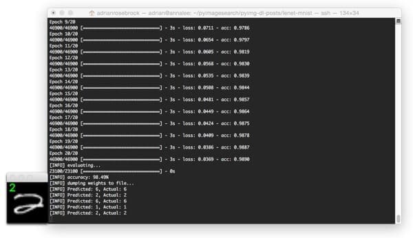
I’ve included the output from my machine below:

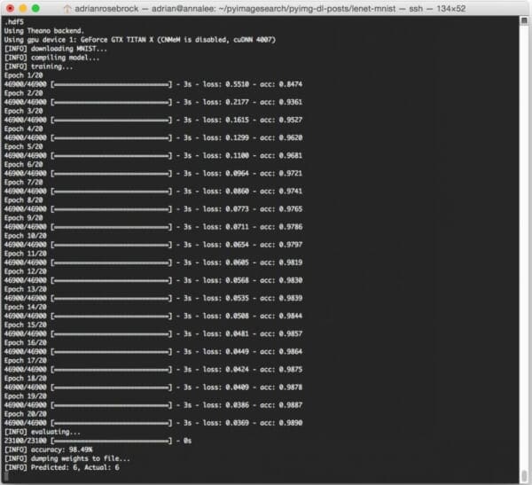
On my Titan X GPU, it takes approximately 3 seconds per epoch, allowing the entire training process to finish in approximately 60 seconds.

After only 20 epochs, LeNet is reaching 98.49% classification accuracy on the MNIST dataset — not bad at all for only 60 seconds of computation time!

Note: If you execute the lenet_mnist.py script on our CPU rather than GPU, expect the per-epoch time to jump to 70-90 seconds. It’s still possible to train LeNet on your CPU, it will just take a little while longer.

Evaluating LeNet with Python and Keras

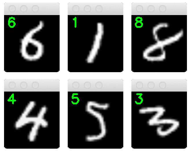
Below I have included a few example evaluation images from our LeNet + MNIST implementation:

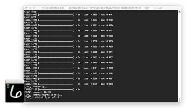
In the above image, we are able to correctly classify the digit as “6”.

And in this image, LeNet correctly recognizes the digit as a “2”:

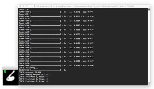
The image below is a great example of the robust, discriminating nature of convolution filters learned by CNN filters: This “6” is quite contorted, leaving little-to-no gap between the circular region of the digit, but LeNet is still able to correctly classify the digit:

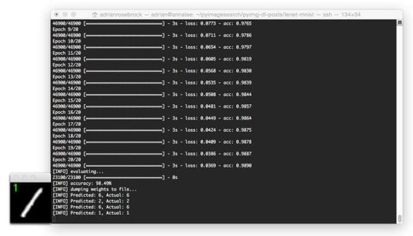
Here is another image, this time classifying a heavily skewed “1”:

Finally, this last example demonstrates the LeNet model classifying a “2”:

Running the serialized LeNet model

After our lenet_mnist.py script finishes executing the first time (provided you supplied both --save-model and --weights ), you should now have a lenet_weights.hdf5 file in your output directory.

Instead of re-training our network on subsequent runs of lenet_mnist.py , we can instead load these weights and use them to classify digits.

To load our pre-trained LeNet model, just execute the following command:

$ python lenet_mnist.py --load-model 1 --weights output/lenet_weights.hdf5

I’ve included a GIF animation of LeNet used to correctly classify handwritten digits below:

Summary

In today’s blog post, I demonstrated how to implement the LeNet architecture using the Python programming language and the Keras library for deep learning.

The LeNet architecture is a great “Hello, World” network to get your feet wet with deep learning and Convolutional Neural Networks. The network itself is simple, has a small memory footprint, and when applied to the MNIST dataset, can be run on either your CPU or GPU, making it ideal for experimenting and learning, especially if you’re a deep learning newcomer.

This tutorial was primarily code focused, and because of this, I needed to skip over detailed reviews of important Convolutional Neural Network concepts such as activation layers, pooling layers, and dense/fully-connected layers (otherwise this post could have easily been 5x as long).

In future blog posts, I’ll be reviewing each of these layer types in lots of detail — in the meantime, simply familiarize yourself with the code and try executing it yourself. And if you’re feeling really daring, try tweaking the number of filters and filter sizes per convolutional layer and see what happens!

Anyway, I hope you’ve enjoyed this blog post — I’ll certainly be doing more deep learning and image classification posts in the future.

But before you go, be sure to enter your email address in the form below to be notified when future PyImageSearch blog posts are published — you won’t want to miss them!