Well. I’ll just come right out and say it. Today is my 27th birthday.
As a kid I was always super excited about my birthday. It was another year closer to being able to drive a car. Go to R rated movies. Or buy alcohol.
But now as an adult, I don’t care too much for my birthday — I suppose it’s just another reminder of the passage of time and how it can’t be stopped. And to be totally honest with you, I guess I’m a bit nervous about turning the “Big 3-0” in a few short years.
In order to rekindle some of that “little kid excitement”, I want to do something special with today’s post. Since today is both a Monday (when new PyImageSearch blog posts are published) and my birthday (two events that will not coincide again until 2020), I’ve decided to put together a really great tutorial on texture and pattern recognition in images.
In the remainder of this blog post I’ll show you how to use the Local Binary Patterns image descriptor (along with a bit of machine learning) to automatically classify and identify textures and patterns in images (such as the texture/pattern of wrapping paper, cake icing, or candles, for instance).
Read on to find out more about Local Binary Patterns and how they can be used for texture classification.
PyImageSearch Gurus
The majority of this blog post on texture and pattern recognition is based on the Local Binary Patterns lesson inside the PyImageSearch Gurus course.
While the lesson in PyImageSearch Gurus goes into a lot more detail than what this tutorial does, I still wanted to give you a taste of what PyImageSearch Gurus — my magnum opus on computer vision — has in store for you.
If you like this tutorial, there are over 29 lessons spanning 324 pages covering image descriptors (HOG, Haralick, Zernike, etc.), keypoint detectors (FAST, DoG, GFTT, etc.), and local invariant descriptors (SIFT, SURF, RootSIFT, etc.), inside the course.
At the time of this writing, the PyImageSearch Gurus course also covers an additional 166 lessons and 1,291 pages including computer vision topics such as face recognition, deep learning, automatic license plate recognition, and training your own custom object detectors, just to name a few.
If this sounds interesting to you, be sure to take a look and consider signing up for the next open enrollment!
What are Local Binary Patterns?
Local Binary Patterns, or LBPs for short, are a texture descriptor made popular by the work of Ojala et al. in their 2002 paper, Multiresolution Grayscale and Rotation Invariant Texture Classification with Local Binary Patterns (although the concept of LBPs were introduced as early as 1993).
Unlike Haralick texture features that compute a global representation of texture based on the Gray Level Co-occurrence Matrix, LBPs instead compute a local representation of texture. This local representation is constructed by comparing each pixel with its surrounding neighborhood of pixels.
The first step in constructing the LBP texture descriptor is to convert the image to grayscale. For each pixel in the grayscale image, we select a neighborhood of size r surrounding the center pixel. A LBP value is then calculated for this center pixel and stored in the output 2D array with the same width and height as the input image.
For example, let’s take a look at the original LBP descriptor which operates on a fixed 3 x 3 neighborhood of pixels just like this:
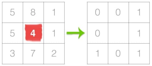
In the above figure we take the center pixel (highlighted in red) and threshold it against its neighborhood of 8 pixels. If the intensity of the center pixel is greater-than-or-equal to its neighbor, then we set the value to 1; otherwise, we set it to 0. With 8 surrounding pixels, we have a total of 2 ^ 8 = 256 possible combinations of LBP codes.
From there, we need to calculate the LBP value for the center pixel. We can start from any neighboring pixel and work our way clockwise or counter-clockwise, but our ordering must be kept consistent for all pixels in our image and all images in our dataset. Given a 3 x 3 neighborhood, we thus have 8 neighbors that we must perform a binary test on. The results of this binary test are stored in an 8-bit array, which we then convert to decimal, like this:

In this example we start at the top-right point and work our way clockwise accumulating the binary string as we go along. We can then convert this binary string to decimal, yielding a value of 23.
This value is stored in the output LBP 2D array, which we can then visualize below:
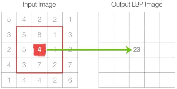
This process of thresholding, accumulating binary strings, and storing the output decimal value in the LBP array is then repeated for each pixel in the input image.
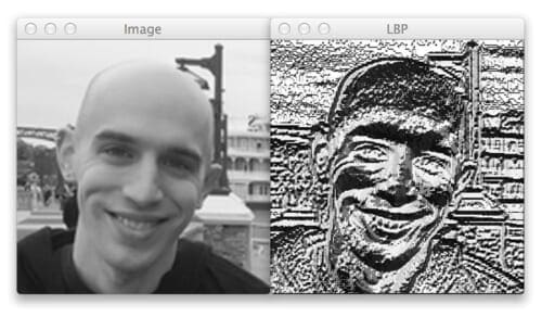
Here is an example of computing and visualizing a full LBP 2D array:
The last step is to compute a histogram over the output LBP array. Since a 3 x 3 neighborhood has 2 ^ 8 = 256 possible patterns, our LBP 2D array thus has a minimum value of 0 and a maximum value of 255, allowing us to construct a 256-bin histogram of LBP codes as our final feature vector:

A primary benefit of this original LBP implementation is that we can capture extremely fine-grained details in the image. However, being able to capture details at such a small scale is also the biggest drawback to the algorithm — we cannot capture details at varying scales, only the fixed 3 x 3 scale!
To handle this, an extension to the original LBP implementation was proposed by Ojala et al. to handle variable neighborhood sizes. To account for variable neighborhood sizes, two parameters were introduced:
- The number of points p in a circularly symmetric neighborhood to consider (thus removing relying on a square neighborhood).
- The radius of the circle r, which allows us to account for different scales.
Below follows a visualization of these parameters:

Lastly, it’s important that we consider the concept of LBP uniformity. A LBP is considered to be uniform if it has at most two 0-1 or 1-0 transitions. For example, the pattern 00001000 (2 transitions) and 10000000 (1 transition) are both considered to be uniform patterns since they contain at most two 0-1 and 1-0 transitions. The pattern 01010010 ) on the other hand is not considered a uniform pattern since it has six 0-1 or 1-0 transitions.
The number of uniform prototypes in a Local Binary Pattern is completely dependent on the number of points p. As the value of p increases, so will the dimensionality of your resulting histogram. Please refer to the original Ojala et al. paper for the full explanation on deriving the number of patterns and uniform patterns based on this value. However, for the time being simply keep in mind that given the number of points p in the LBP there are p + 1 uniform patterns. The final dimensionality of the histogram is thus p + 2, where the added entry tabulates all patterns that are not uniform.
So why are uniform LBP patterns so interesting? Simply put: they add an extra level of rotation and grayscale invariance, hence they are commonly used when extracting LBP feature vectors from images.
Local Binary Patterns with Python and OpenCV
Local Binary Pattern implementations can be found in both the scikit-image and mahotas packages. OpenCV also implements LBPs, but strictly in the context of face recognition — the underlying LBP extractor is not exposed for raw LBP histogram computation.
In general, I recommend using the scikit-image implementation of LBPs as they offer more control of the types of LBP histograms you want to generate. Furthermore, the scikit-image implementation also includes variants of LBPs that improve rotation and grayscale invariance.
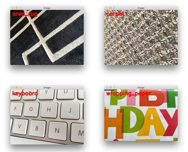
Before we get started extracting Local Binary Patterns from images and using them for classification, we first need to create a dataset of textures. To form this dataset, earlier today I took a walk through my apartment and collected 20 photos of various textures and patterns, including an area rug:

Notice how the area rug images have a geometric design to it.
I also gathered a few examples of carpet:

Notice how the carpet has a distinct pattern with a coarse texture.
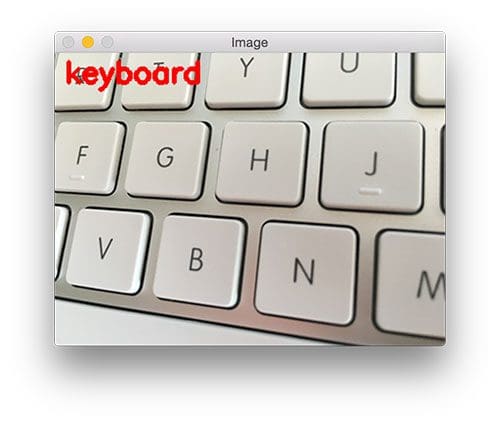
I then snapped a few photos of the keyboard sitting on my desk:

Notice how the keyboard has little texture — but it does demonstrate a repeatable pattern of white keys and silver metal spacing in between them.
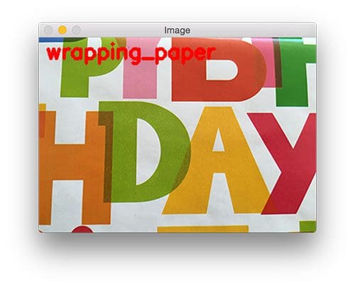
Finally, I gathered a few final examples of wrapping paper (since it is my birthday after all):

The wrapping paper has a very smooth texture to it, but also demonstrates a unique pattern.
Given this dataset of area rug, carpet, keyboard, and wrapping paper, our goal is to extract Local Binary Patterns from these images and apply machine learning to automatically recognize and categorize these texture images.
Let’s go ahead and get this demonstration started by defining the directory structure for our project:
$ tree --dirsfirst -L 3
.
├── images
│   ├── testing
│   │   ├── area_rug.png
│   │   ├── carpet.png
│   │   ├── keyboard.png
│   │   └── wrapping_paper.png
│   └── training
│       ├── area_rug [4 entries]
│       ├── carpet [4 entries]
│       ├── keyboard [4 entries]
│       └── wrapping_paper [4 entries]
├── pyimagesearch
│   ├── __init__.py
│   └── localbinarypatterns.py
└── recognize.py

8 directories, 7 files
The images/ directory contains our testing/ and training/ images.
We’ll be creating a pyimagesearch module to keep our code organized. And within the pyimagesearch module we’ll create localbinarypatterns.py , which as the name suggests, is where our Local Binary Patterns implementation will be stored.
Speaking of Local Binary Patterns, let’s go ahead and create the descriptor class now:
# import the necessary packages
from skimage import feature
import numpy as np

class LocalBinaryPatterns:
	def __init__(self, numPoints, radius):
		# store the number of points and radius
		self.numPoints = numPoints
		self.radius = radius

	def describe(self, image, eps=1e-7):
		# compute the Local Binary Pattern representation
		# of the image, and then use the LBP representation
		# to build the histogram of patterns
		lbp = feature.local_binary_pattern(image, self.numPoints,
			self.radius, method="uniform")
		(hist, _) = np.histogram(lbp.ravel(),
			bins=np.arange(0, self.numPoints + 3),
			range=(0, self.numPoints + 2))

		# normalize the histogram
		hist = hist.astype("float")
		hist /= (hist.sum() + eps)

		# return the histogram of Local Binary Patterns
		return hist
We start of by importing the feature sub-module of scikit-image which contains the implementation of the Local Binary Patterns descriptor.
Line 5 defines our constructor for our LocalBinaryPatterns class. As mentioned in the section above, we know that LBPs require two parameters: the radius of the pattern surrounding the central pixel, along with the number of points along the outer radius. We’ll store both of these values on Lines 8 and 9.
From there, we define our describe method on Line 11, which accepts a single required argument — the image we want to extract LBPs from.
The actual LBP computation is handled on Lines 15 and 16 using our supplied radius and number of points. The uniform method indicates that we are computing the rotation and grayscale invariant form of LBPs.
However, the lbp variable returned by the local_binary_patterns function is not directly usable as a feature vector. Instead, lbp is a 2D array with the same width and height as our input image — each of the values inside lbp ranges from [0, numPoints + 2], a value for each of the possible numPoints + 1 possible rotation invariant prototypes (see the discussion of uniform patterns at the top of this post for more information) along with an extra dimension for all patterns that are not uniform, yielding a total of numPoints + 2 unique possible values.
Thus, to construct the actual feature vector, we need to make a call to np.histogram which counts the number of times each of the LBP prototypes appears. The returned histogram is numPoints + 2-dimensional, an integer count for each of the prototypes. We then take this histogram and normalize it such that it sums to 1, and then return it to the calling function.
Now that our LocalBinaryPatterns descriptor is defined, let’s see how we can use it to recognize textures and patterns. Create a new file named recognize.py , and let’s get coding:
# import the necessary packages
from pyimagesearch.localbinarypatterns import LocalBinaryPatterns
from sklearn.svm import LinearSVC
from imutils import paths
import argparse
import cv2
import os

# construct the argument parse and parse the arguments
ap = argparse.ArgumentParser()
ap.add_argument("-t", "--training", required=True,
	help="path to the training images")
ap.add_argument("-e", "--testing", required=True,
	help="path to the tesitng images")
args = vars(ap.parse_args())

# initialize the local binary patterns descriptor along with
# the data and label lists
desc = LocalBinaryPatterns(24, 8)
data = []
labels = []
We start off on Lines 2-7 by importing our necessary command line arguments. Notice how we are importing the LocalBinaryPatterns descriptor from the pyimagesearch sub-module that we defined above.
From there, Lines 10-15 handle parsing our command line arguments. We’ll only need two switches here: the path to the --training data and the path to the --testing data.
In this example, we have partitioned our textures into two sets: a training set of 4 images per texture (4 textures x 4 images per texture = 16 total images), and a testing set of one image per texture (4 textures x 1 image per texture = 4 images). The training set of 16 images will be used to “teach” our classifier — and then we’ll evaluate performance on our testing set of 4 images.
On Line 19 we initialize our LocalBinaryPattern descriptor using a numPoints=24 and radius=8.
In order to store the LBP feature vectors and the label names associated with each of the texture classes, we’ll initialize two lists: data to store the feature vectors and labels to store the names of each texture (Lines 20 and 21).
Now it’s time to extract LBP features from our set of training images:
# loop over the training images
for imagePath in paths.list_images(args["training"]):
	# load the image, convert it to grayscale, and describe it
	image = cv2.imread(imagePath)
	gray = cv2.cvtColor(image, cv2.COLOR_BGR2GRAY)
	hist = desc.describe(gray)

	# extract the label from the image path, then update the
	# label and data lists
	labels.append(imagePath.split(os.path.sep)[-2])
	data.append(hist)

# train a Linear SVM on the data
model = LinearSVC(C=100.0, random_state=42)
model.fit(data, labels)
We start looping over our training images on Line 24. For each of these images, we load them from disk, convert them to grayscale, and extract Local Binary Pattern features. The label (i.e., texture name) is then extracted from the image path and both our labels and data lists are updated, respectively.
Once we have our features and labels extracted, we can train our Linear Support Vector Machine on Lines 36 and 37 to learn the difference between the various texture classes.
Once our Linear SVM is trained, we can use it to classify subsequent texture images:
# loop over the testing images
for imagePath in paths.list_images(args["testing"]):
	# load the image, convert it to grayscale, describe it,
	# and classify it
	image = cv2.imread(imagePath)
	gray = cv2.cvtColor(image, cv2.COLOR_BGR2GRAY)
	hist = desc.describe(gray)
	prediction = model.predict(hist.reshape(1, -1))

	# display the image and the prediction
	cv2.putText(image, prediction[0], (10, 30), cv2.FONT_HERSHEY_SIMPLEX,
		1.0, (0, 0, 255), 3)
	cv2.imshow("Image", image)
	cv2.waitKey(0)
Just as we looped over the training images on Line 24 to gather data to train our classifier, we now loop over the testing images on Line 40 to test the performance and accuracy of our classifier.
Again, all we need to do is load our image from disk, convert it to grayscale, extract Local Binary Patterns from the grayscale image, and then pass the features onto our Linear SVM for classification (Lines 43-46).
I’d like to draw your attention to hist.reshape(1, -1) on Line 46. This reshapes our histogram from a 1D array to a 2D array allowing for the potential of multiple feature vectors to run predictions on.
Lines 49-52 show the output classification to our screen.
Results
Let’s go ahead and give our texture classification system a try by executing the following command:
$ python recognize.py --training images/training --testing images/testing
And here’s the first output image from our classification:
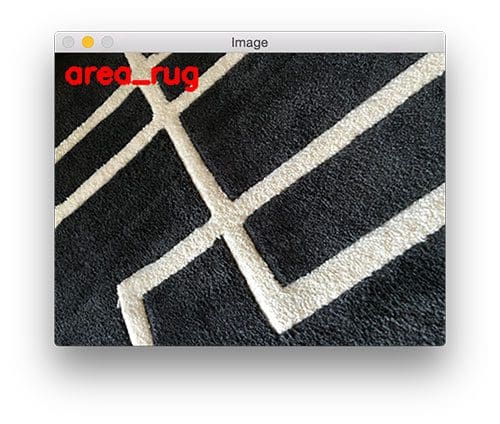
Sure enough, the image is correctly classified as “area rug”.
Let’s try another one:
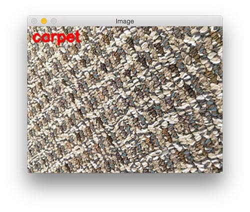
Once again, our classifier correctly identifies the texture/pattern of the image.
Here’s an example of the keyboard pattern being correctly labeled:
Finally, we are able to recognize the texture and pattern of the wrapping paper as well:
While this example was quite small and simple, it was still able to demonstrate that by using Local Binary Pattern features and a bit of machine learning, we are able to correctly classify the texture and pattern of an image.
What's next? We recommend PyImageSearch University.
86+ total classes • 115+ hours hours of on-demand code walkthrough videos • Last updated: April 2026
★★★★★ 4.84 (128 Ratings) • 16,000+ Students Enrolled
I strongly believe that if you had the right teacher you could master computer vision and deep learning.
Do you think learning computer vision and deep learning has to be time-consuming, overwhelming, and complicated? Or has to involve complex mathematics and equations? Or requires a degree in computer science?
That’s not the case.
All you need to master computer vision and deep learning is for someone to explain things to you in simple, intuitive terms. And that’s exactly what I do. My mission is to change education and how complex Artificial Intelligence topics are taught.
If you're serious about learning computer vision, your next stop should be PyImageSearch University, the most comprehensive computer vision, deep learning, and OpenCV course online today. Here you’ll learn how to successfully and confidently apply computer vision to your work, research, and projects. Join me in computer vision mastery.
Inside PyImageSearch University you'll find:
- ✓ 86+ courses on essential computer vision, deep learning, and OpenCV topics
- ✓ 86 Certificates of Completion
- ✓ 115+ hours hours of on-demand video
- ✓ Brand new courses released regularly, ensuring you can keep up with state-of-the-art techniques
- ✓ Pre-configured Jupyter Notebooks in Google Colab
- ✓ Run all code examples in your web browser — works on Windows, macOS, and Linux (no dev environment configuration required!)
- ✓ Access to centralized code repos for all 540+ tutorials on PyImageSearch
- ✓ Easy one-click downloads for code, datasets, pre-trained models, etc.
- ✓ Access on mobile, laptop, desktop, etc.
Summary
In this blog post we learned how to extract Local Binary Patterns from images and use them (along with a bit of machine learning) to perform texture and pattern recognition.
If you enjoyed this blog post, be sure to take a look at the PyImageSearch Gurus course where the majority this lesson was derived from.
Inside the course you’ll find over 166+ lessons covering 1,291 pages of computer vision topics such as:
- Face recognition.
- Deep learning.
- Automatic license plate recognition.
- Training your own custom object detectors.
- Building image search engines.
- …and much more!
If this sounds interesting to you, be sure to take a look and consider signing up for the next open enrollment!
See you next week!

Download the Source Code and FREE 17-page Resource Guide
Enter your email address below to get a .zip of the code and a FREE 17-page Resource Guide on Computer Vision, OpenCV, and Deep Learning. Inside you'll find my hand-picked tutorials, books, courses, and libraries to help you master CV and DL!
