Today’s blog post wouldn’t be possible without PyImageSearch Gurus member, Hans Boone. Hans is working on a computer vision project to automatically detect Machine-readable Zones (MRZs) in passport images — much like the region detected in the image above.
The MRZ region in passports or travel cards fall into two classes: Type 1 and Type 3. Type 1 MRZs are three lines, with each line containing 30 characters. The Type 3 MRZ only has two lines, but each line contains 44 characters. In either case, the MRZ encodes identifying information of a given citizen, including the type of passport, passport ID, issuing country, name, nationality, expiration date, etc.
Inside the PyImageSearch Gurus course, Hans showed me his progress on the project and I immediately became interested. I’ve always wanted to apply computer vision algorithms to passport images (mainly just for fun), but lacked the dataset to do so. Given the personal identifying information a passport contains, I obviously couldn’t write a blog post on the subject and share the images I used to develop the algorithm.
Luckily, Hans agreed to share some of the sample/specimen passport images he has access to — and I jumped at the chance to play with these images.
Now, before we get to far, it’s important to note that these passports are not “real” in the sense that they can be linked to an actual human being. But they are genuine passports that were generated using fake names, addresses, etc. for developers to work with.
You might think that in order to detect the MRZ region of a passport that you need a bit of machine learning, perhaps using the Linear SVM + HOG framework to construct an “MRZ detector” — but that would be overkill.
Instead, we can perform MRZ detection using only basic image processing techniques such as thresholding, morphological operations, and contour properties. In the remainder of this blog post, I’ll detail my own take on how to apply these methods to detect the MRZ region of a passport.
Detecting machine-readable zones in passport images
Let’s go ahead and get this project started. Open up a new file, name it detect_mrz.py , and insert the following code:
# import the necessary packages
from imutils import paths
import numpy as np
import argparse
import imutils
import cv2

# construct the argument parse and parse the arguments
ap = argparse.ArgumentParser()
ap.add_argument("-i", "--images", required=True, help="path to images directory")
args = vars(ap.parse_args())

# initialize a rectangular and square structuring kernel
rectKernel = cv2.getStructuringElement(cv2.MORPH_RECT, (13, 5))
sqKernel = cv2.getStructuringElement(cv2.MORPH_RECT, (21, 21))
Lines 2-6 import our necessary packages. I’ll assume you already have OpenCV installed. You’ll also need imutils, my collection of convenience functions to make basic image processing operations with OpenCV easier. You can install imutils using pip :
$ pip install --upgrade imutils
From there, Lines 9-11 handle parsing our command line argument. We only need a single switch here, --images , which is the path to the directory containing the passport images we are going to process.
Finally, Lines 14 and 15 initialize two kernels which we’ll later use when applying morphological operations, specifically the closing operation. For the time being, simply note that the first kernel is rectangular with a width approximately 3x larger than the height. The second kernel is square. These kernels will allow us to close gaps between MRZ characters and openings between MRZ lines.
Now that our command line arguments are parsed, we can start looping over each of the images in our dataset and process them:
# loop over the input image paths
for imagePath in paths.list_images(args["images"]):
	# load the image, resize it, and convert it to grayscale
	image = cv2.imread(imagePath)
	image = imutils.resize(image, height=600)
	gray = cv2.cvtColor(image, cv2.COLOR_BGR2GRAY)

	# smooth the image using a 3x3 Gaussian, then apply the blackhat
	# morphological operator to find dark regions on a light background
	gray = cv2.GaussianBlur(gray, (3, 3), 0)
	blackhat = cv2.morphologyEx(gray, cv2.MORPH_BLACKHAT, rectKernel)
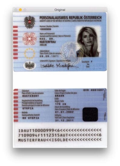
Lines 20 and 21 loads our original image from disk and resizes it to have a maximum height of 600 pixels. You can see an example of an original image below:
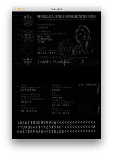
Gaussian blurring is applied on Line 26 to reduce high frequency noise. We then apply a blackhat morphological operation to the blurred, grayscale image on Line 27.
A blackhat operator is used to reveal dark regions (i.e., MRZ text) against light backgrounds (i.e., the background of the passport itself). Since the passport text is always black on a light background (at least in terms of this dataset), a blackhat operation is appropriate. Below you can see the output of applying the blackhat operator:
The next step in MRZ detection is to compute the gradient magnitude representation of the blackhat image using the Scharr operator:
	# compute the Scharr gradient of the blackhat image and scale the
	# result into the range [0, 255]
	gradX = cv2.Sobel(blackhat, ddepth=cv2.CV_32F, dx=1, dy=0, ksize=-1)
	gradX = np.absolute(gradX)
	(minVal, maxVal) = (np.min(gradX), np.max(gradX))
	gradX = (255 * ((gradX - minVal) / (maxVal - minVal))).astype("uint8")
Here we compute the Scharr gradient along the x-axis of the blackhat image, revealing regions of the image that are not only dark against a light background, but also contain vertical changes in the gradient, such as the MRZ text region. We then take this gradient image and scale it back into the range [0, 255] using min/max scaling:

While it isn’t entirely obvious why we apply this step, I will say that it’s extremely helpful in reducing false-positive MRZ detections. Without it, we can accidentally mark embellished or designed regions of the passport as the MRZ. I will leave this as an exercise to you to verify that computing the gradient of the blackhat image can improve MRZ detection accuracy.
The next step is to try to detect the actual lines of the MRZ:
	# apply a closing operation using the rectangular kernel to close
	# gaps in between letters -- then apply Otsu's thresholding method
	gradX = cv2.morphologyEx(gradX, cv2.MORPH_CLOSE, rectKernel)
	thresh = cv2.threshold(gradX, 0, 255, cv2.THRESH_BINARY | cv2.THRESH_OTSU)[1]
First, we apply a closing operation using our rectangular kernel. This closing operation is meant to close gaps in between MRZ characters. We then apply thresholding using Otsu’s method to automatically threshold the image:
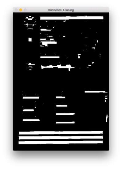
As we can see from the figure above, each of the MRZ lines is present in our threshold map.
The next step is to close the gaps between the actual lines, giving us one large rectangular region that corresponds to the MRZ:
	# perform another closing operation, this time using the square
	# kernel to close gaps between lines of the MRZ, then perform a
	# series of erosions to break apart connected components
	thresh = cv2.morphologyEx(thresh, cv2.MORPH_CLOSE, sqKernel)
	thresh = cv2.erode(thresh, None, iterations=4)
Here we perform another closing operation, this time using our square kernel. This kernel is used to close gaps between the individual lines of the MRZ, giving us one large region that corresponds to the MRZ. A series of erosions are then performed to break apart connected components that may have been joined during the closing operation. These erosions are also helpful in removing small blobs that are irrelevant to the MRZ.

For some passport scans, the border of the passport may have become attached to the MRZ region during the closing operations. To remedy this, we set 5% of the left and right borders of the image to zero (i.e., black):
	# during thresholding, it's possible that border pixels were
	# included in the thresholding, so let's set 5% of the left and
	# right borders to zero
	p = int(image.shape[1] * 0.05)
	thresh[:, 0:p] = 0
	thresh[:, image.shape[1] - p:] = 0
You can see the output of our border removal below.
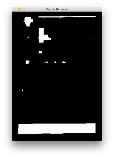
Compared to Figure 5 above, you can now see that the border has been removed.
The last step is to find the contours in our thresholded image and use contour properties to identify the MRZ:
	# find contours in the thresholded image and sort them by their
	# size
	cnts = cv2.findContours(thresh.copy(), cv2.RETR_EXTERNAL,
		cv2.CHAIN_APPROX_SIMPLE)
	cnts = imutils.grab_contours(cnts)
	cnts = sorted(cnts, key=cv2.contourArea, reverse=True)

	# loop over the contours
	for c in cnts:
		# compute the bounding box of the contour and use the contour to
		# compute the aspect ratio and coverage ratio of the bounding box
		# width to the width of the image
		(x, y, w, h) = cv2.boundingRect(c)
		ar = w / float(h)
		crWidth = w / float(gray.shape[1])

		# check to see if the aspect ratio and coverage width are within
		# acceptable criteria
		if ar > 5 and crWidth > 0.75:
			# pad the bounding box since we applied erosions and now need
			# to re-grow it
			pX = int((x + w) * 0.03)
			pY = int((y + h) * 0.03)
			(x, y) = (x - pX, y - pY)
			(w, h) = (w + (pX * 2), h + (pY * 2))

			# extract the ROI from the image and draw a bounding box
			# surrounding the MRZ
			roi = image[y:y + h, x:x + w].copy()
			cv2.rectangle(image, (x, y), (x + w, y + h), (0, 255, 0), 2)
			break

	# show the output images
	cv2.imshow("Image", image)
	cv2.imshow("ROI", roi)
	cv2.waitKey(0)
On Line 56-58 we compute the contours (i.e., outlines) of our thresholded image. We then take these contours and sort them based on their size in descending order on Line 59 (implying that the largest contours are first in the list).
On Line 62 we start looping over our sorted list of contours. For each of these contours, we’ll compute the bounding box (Line 66) and use it to compute two properties: the aspect ratio and the coverage ratio. The aspect ratio is simply the width of the bounding box divided by the height. The coverage ratio is the width of the bounding box divided by the width of the actual image.
Using these two properties we can make a check on Line 72 to see if we are examining the MRZ region. The MRZ is rectangular, with a width that is much larger than the height. The MRZ should also span at least 75% of the input image.
Provided these two cases hold, Lines 75-84 use the (x, y)-coordinates of the bounding box to extract the MRZ and draw the bounding box on our input image.
Finally, Lines 87-89 display our results.
Results
To see our MRZ detector in action, just execute the following command:
$ python detect_mrz.py --images examples
Below you can see of an example of a successful MRZ detection, with the MRZ outlined in green:

Here is another example of detecting the Machine-readable Zone in a passport image using Python and OpenCV:
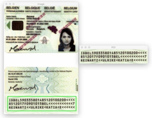
It doesn’t matter if the MRZ region is at the top or the bottom of the image. By applying morphological operations, extracting contours, and computing contour properties, we are able to extract the MRZ without a problem.
The same is true for the following image:

Let’s give another image a try:
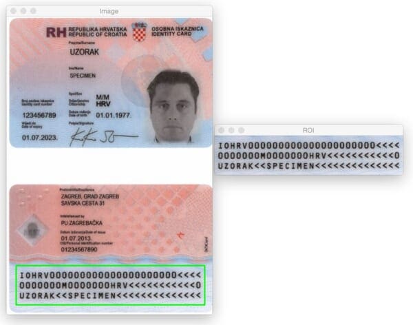
Up until now we have only seen Type 1 MRZs that contain three lines. However, our method works just as well with Type 3 MRZs that contain only two lines:

Here’s another example of detecting a Type 3 MRZ:

What's next? We recommend PyImageSearch University.
86+ total classes • 115+ hours hours of on-demand code walkthrough videos • Last updated: May 2026
★★★★★ 4.84 (128 Ratings) • 16,000+ Students Enrolled
I strongly believe that if you had the right teacher you could master computer vision and deep learning.
Do you think learning computer vision and deep learning has to be time-consuming, overwhelming, and complicated? Or has to involve complex mathematics and equations? Or requires a degree in computer science?
That’s not the case.
All you need to master computer vision and deep learning is for someone to explain things to you in simple, intuitive terms. And that’s exactly what I do. My mission is to change education and how complex Artificial Intelligence topics are taught.
If you're serious about learning computer vision, your next stop should be PyImageSearch University, the most comprehensive computer vision, deep learning, and OpenCV course online today. Here you’ll learn how to successfully and confidently apply computer vision to your work, research, and projects. Join me in computer vision mastery.
Inside PyImageSearch University you'll find:
- ✓ 86+ courses on essential computer vision, deep learning, and OpenCV topics
- ✓ 86 Certificates of Completion
- ✓ 115+ hours hours of on-demand video
- ✓ Brand new courses released regularly, ensuring you can keep up with state-of-the-art techniques
- ✓ Pre-configured Jupyter Notebooks in Google Colab
- ✓ Run all code examples in your web browser — works on Windows, macOS, and Linux (no dev environment configuration required!)
- ✓ Access to centralized code repos for all 540+ tutorials on PyImageSearch
- ✓ Easy one-click downloads for code, datasets, pre-trained models, etc.
- ✓ Access on mobile, laptop, desktop, etc.
Summary
In this blog post we learned how to detect Machine-readable Zones (MRZs) in passport scans using only basic image processing techniques, namely:
- Thresholding.
- Gradients.
- Morphological operations (specifically, closings and erosions).
- Contour properties.
These operations, while simple, allowed us to detect the MRZ regions in images without having to rely on more advanced feature extraction and machine learning methods such as Linear SVM + HOG for object detection.
Remember, when faced with a challenging computer vision problem — always consider the problem and your assumptions! As this blog post demonstrates, you might be surprised what basic image processing functions used in tandem can accomplish.
Once again, a big thanks to PyImageSearch Gurus member, Hans Boone, who supplied us with these example passport images! Thanks Hans!

Download the Source Code and FREE 17-page Resource Guide
Enter your email address below to get a .zip of the code and a FREE 17-page Resource Guide on Computer Vision, OpenCV, and Deep Learning. Inside you'll find my hand-picked tutorials, books, courses, and libraries to help you master CV and DL!

