Training a DCGAN in PyTorch

In this tutorial, we will learn how to train our first DCGAN Model using PyTorch to generate images.

This lesson is part 1 of a 3-part series on Advanced PyTorch Techniques:

1. Training a DCGAN in PyTorch (today’s tutorial)
2. Training an object detector from scratch in PyTorch (next week’s lesson)
3. U-Net: Training Image Segmentation Models in PyTorch (in 2 weeks)

By 2014, the world of Machine Learning had already made quite significant strides. Several new concepts (like Attention and R-CNN) were being introduced. However, the idea of machine learning had been shaped so that they were all expected in some way or another.

That is until Ian Goodfellow et al. wrote a paper that changed the world of machine learning; Generative Adversarial Networks.

After the success of deep convolutional networks in the image domain, it wasn’t long until the idea was integrated with GANs. As a result, DCGANs were born.

To learn how to generate images using DCGAN written in PyTorch, just keep reading.

Training a DCGAN in PyTorch

Structure of the tutorial:

• Intro to GANs and DCGANs
• Understanding the DCGAN Architecture
• PyTorch Implementation and Walkthrough
• Suggestions on what to try next

Generative Adversarial Networks

The distinguishing factor of GANs is their ability to generate authentic, real-looking images, similar to the data distribution you might use.

The concept of GANs is simple yet ingenious. Let’s try and understand the concept using a simple example (Figure 1).

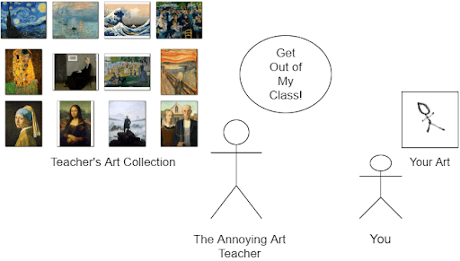
You recently enrolled in an art class, where the art teacher is extremely harsh and strict. When you hand in your first painting, the art teacher is aghast. He threatens to have you expelled until you can make a spectacular masterpiece.

Needless to say, you are upset. The task is incredibly difficult, seeing how you’re just a fledgling. The only thing going for you is that your annoying art teacher said that the masterpiece doesn’t have to be a direct replica of his collections, but it has to look like it belongs up there with them.

You anxiously start bettering your art. Over the next few days, you submit a few trial copies, each better than your last attempt but not good enough to get you through this test.

All this while, your art teacher also starts becoming a better judge of the paintings shown to him. With just a glance, he can name the artists and artworks you’re attempting to replicate. Finally, the day of reckoning arrives, and you submit your final work (Figure 2).

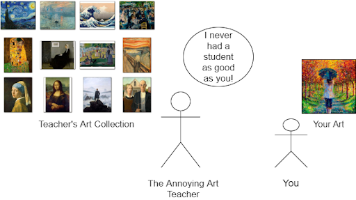
You come up with a painting so good that your art teacher places it amongst his collection. He praises you and accepts you as a full-time student (but by that time, you realize you don’t need him anymore).

A GAN works in the same way. “You” are the Generator who is trying to generate images mimicking a given input dataset. While the “art teacher” is the Discriminator, whose job is to judge if the image you generated can be grouped with the input dataset or not. The only difference between the above example and a GAN is that both the generator and the discriminator are trained together from scratch.

These networks provide feedback to each other, and as we train the GAN model, both improve, and we get better quality in our output images.

For a complete tutorial on implementing a GAN model in Keras and Tensorflow, I recommend this tutorial by Adrian Rosebrock.

What Are DCGANs?

Radford et al. (2016) published a paper on Deep Convolutional Generative Adversarial Networks (DCGANs).

DCGANs at that time showed us how to effectively use Convolutional techniques with GANs without supervision to create images that are quite similar to those in our dataset.

In this post, I will explain DCGANs and their key research introductions and walk you through a PyTorch implementation of the same on the MNIST dataset. As a side note, this is really cool since one of the paper’s co-authors is Soumith Chintala, a core creator of PyTorch!

DCGANs Architecture

Let’s dive into the architecture:

Figure 3 contains the architecture of the generator used in DCGAN, as shown in the paper.

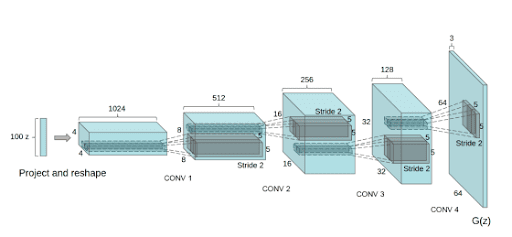
As seen in Figure 3, we are taking a random noise vector as input and giving a complete image as the output. Let’s look at the discriminator architecture in Figure 4.

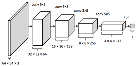
The Discriminator is acting as a normal deterministic model, whose job is to classify an input image as real or fake.

The paper’s authors have created a different section explaining the differences between their approach and a vanilla GAN.

• The pooling layers of a vanilla GAN are replaced by fractionally strided convolutions (in the case of the Generator) and strided convolutions (in the case of the Discriminator). For the former, I definitely recommend this video tutorial by Sebastian Raschka. Fractionally strided convolutions were an alternative to standard upscaling, allowing the model to learn its own spatial representations instead of having non-trainable deterministic pooling layers.
• The second most important deviation from vanilla GANs is the exclusion of fully connected layers in favor of deeper architectures.
• Thirdly, Ioffe and Szegedy (2015) have emphasized the importance of batch normalization to ensure the proper flow of gradients in deeper networks.
• Finally, Radford et al. explain the use of ReLU and leaky ReLU in their architecture, citing the success of bounded functions, to help learn about the training distribution quicker.

Let’s see how these factors affect the results!

Configuring Your Development Environment

To follow this guide, you need to have the OpenCV library installed on your system.

Luckily, OpenCV is pip-installable:

$ pip install opencv-contrib-python

If you need help configuring your development environment for OpenCV, I highly recommend that you read my pip install OpenCV guide — it will have you up and running in a matter of minutes.

Having Problems Configuring Your Development Environment?

All that said, are you:

• Short on time?
• Learning on your employer’s administratively locked system?
• Wanting to skip the hassle of fighting with the command line, package managers, and virtual environments?
• Ready to run the code right now on your Windows, macOS, or Linux system?

Then join PyImageSearch University today!

Gain access to Jupyter Notebooks for this tutorial and other PyImageSearch guides that are pre-configured to run on Google Colab’s ecosystem right in your web browser! No installation required.

And best of all, these Jupyter Notebooks will run on Windows, macOS, and Linux!

Project Structure

We first need to review our project directory structure.

Start by accessing the “Downloads” section of this tutorial to retrieve the source code and example images.

From there, take a look at the directory structure:

!tree .
.
├── dcgan_mnist.py
├── output
│   ├── epoch_0002.png
│   ├── epoch_0004.png
│   ├── epoch_0006.png
│   ├── epoch_0008.png
│   ├── epoch_0010.png
│   ├── epoch_0012.png
│   ├── epoch_0014.png
│   ├── epoch_0016.png
│   ├── epoch_0018.png
│   └── epoch_0020.png
├── output.gif
└── pyimagesearch
    ├── dcgan.py
    └── __init__.py

In the pyimagesearch directory, we have two files:

• dcgan.py: Contains the complete DCGAN architecture
• __init__.py: Turns the pyimagesearch into a python directory

In the parent directory, we have the dcgan_mnist.py script, which will train the DCGAN and draw inference from it.

Apart from these, we have the output directory, which contains the epoch-wise visualization of images generated by the DCGAN Generator. Finally, we have the output.gif, which contains the visualizations converted into a gif.

Implementing the DCGAN in PyTorch

Our first task is to hop into the pyimagesearch directory and open the dcgan.py script. This script will house the complete DCGAN architecture.

# import the necessary packages
from torch.nn import ConvTranspose2d
from torch.nn import BatchNorm2d
from torch.nn import Conv2d
from torch.nn import Linear
from torch.nn import LeakyReLU
from torch.nn import ReLU
from torch.nn import Tanh
from torch.nn import Sigmoid
from torch import flatten
from torch import nn

class Generator(nn.Module):
	def __init__(self, inputDim=100, outputChannels=1):
		super(Generator, self).__init__()

		# first set of CONVT => RELU => BN
		self.ct1 = ConvTranspose2d(in_channels=inputDim,
			out_channels=128, kernel_size=4, stride=2, padding=0,
			bias=False)
		self.relu1 = ReLU()
		self.batchNorm1 = BatchNorm2d(128)

		# second set of CONVT => RELU => BN
		self.ct2 = ConvTranspose2d(in_channels=128, out_channels=64,
					kernel_size=3, stride=2, padding=1, bias=False)
		self.relu2 = ReLU()
		self.batchNorm2 = BatchNorm2d(64)

		# last set of CONVT => RELU => BN
		self.ct3 = ConvTranspose2d(in_channels=64, out_channels=32,
					kernel_size=4, stride=2, padding=1, bias=False)
		self.relu3 = ReLU()
		self.batchNorm3 = BatchNorm2d(32)

		# apply another upsample and transposed convolution, but
		# this time output the TANH activation
		self.ct4 = ConvTranspose2d(in_channels=32,
			out_channels=outputChannels, kernel_size=4, stride=2,
			padding=1, bias=False)
		self.tanh = Tanh()

Here, we have created the Generator class (Line 13). In our __init__ constructor, we have 2 important things to keep in mind (Line 14):

• inputDim: The input size of the noise vector passed through the generator.
• outputChannels: The number of channels of the output image. Since we are using the MNIST dataset, the image will be in grayscale. Hence it’ll have a single channel.

Since PyTorch’s convolutions don’t need height and width specifications, we won’t have to specify the output dimensions apart from the channel size. However, since we’re using MNIST data, we’ll need an output of size 1×28×28.

Remember, the Generator is going to model random noise into an image. Keeping that in mind, our next task is to define the layers of the Generator. We are going to use CONVT (Transposed Convolutions), ReLU (Rectified Linear Units), BN (Batch Normalization) (Lines 18-34). The final transposed convolution will be followed by a tanh activation function, bounding our output pixel values to 1 to -1 (Lines 38-41).

	def forward(self, x):
		# pass the input through our first set of CONVT => RELU => BN
		# layers
		x = self.ct1(x)
		x = self.relu1(x)
		x = self.batchNorm1(x)

		# pass the output from previous layer through our second
		# CONVT => RELU => BN layer set
		x = self.ct2(x)
		x = self.relu2(x)
		x = self.batchNorm2(x)

		# pass the output from previous layer through our last set
		# of CONVT => RELU => BN layers
		x = self.ct3(x)
		x = self.relu3(x)
		x = self.batchNorm3(x)

		# pass the output from previous layer through CONVT2D => TANH
		# layers to get our output
		x = self.ct4(x)
		output = self.tanh(x)

		# return the output
		return output

In the forward pass of the generator, we use the CONVT=> ReLU => BN pattern thrice, while the final CONVT layer is followed by the tanh layer (Lines 46-65).

class Discriminator(nn.Module):
	def __init__(self, depth, alpha=0.2):
		super(Discriminator, self).__init__()

		# first set of CONV => RELU layers
		self.conv1 = Conv2d(in_channels=depth, out_channels=32,
				kernel_size=4, stride=2, padding=1)
		self.leakyRelu1 = LeakyReLU(alpha, inplace=True)

		# second set of CONV => RELU layers
		self.conv2 = Conv2d(in_channels=32, out_channels=64, kernel_size=4,
				stride=2, padding=1)
		self.leakyRelu2 = LeakyReLU(alpha, inplace=True)

		# first (and only) set of FC => RELU layers
		self.fc1 = Linear(in_features=3136, out_features=512)
		self.leakyRelu3 = LeakyReLU(alpha, inplace=True)

		# sigmoid layer outputting a single value
		self.fc2 = Linear(in_features=512, out_features=1)
		self.sigmoid = Sigmoid()

Keep in mind that while the Generator models random noise into an image, the Discriminator takes the image and outputs a single value (determining if it belongs to the input distribution or not).

In the Discriminator’s constructor function __init__, there are just two arguments:

• depth: Determines the number of channels of the input image
• alpha: The value given to the leaky ReLU functions used in the architecture

We initialize a set of convolution layers, leaky ReLU layers, two linear layers followed by a final sigmoid layer (Lines 75-90). The paper‘s authors mention that the leaky ReLU’s property of allowing some value below zero helped the Discriminator’s results. Of course, the final sigmoid layer is to map the singular output value to either 0 or 1.

	def forward(self, x):
		# pass the input through first set of CONV => RELU layers
		x = self.conv1(x)
		x = self.leakyRelu1(x)

		# pass the output from the previous layer through our second
		# set of CONV => RELU layers
		x = self.conv2(x)
		x = self.leakyRelu2(x)

		# flatten the output from the previous layer and pass it
		# through our first (and only) set of FC => RELU layers
		x = flatten(x, 1)
		x = self.fc1(x)
		x = self.leakyRelu3(x)

		# pass the output from the previous layer through our sigmoid
		# layer outputting a single value
		x = self.fc2(x)
		output = self.sigmoid(x)

		# return the output
		return output

In the forward pass of the Discriminator, we first add a convolution layer and a leaky ReLU layer and repeat the pattern once more (Lines 94-100). This is followed by a flatten layer, a fully connected layer, and another leaky ReLU layer (Lines 104-106). Before the final sigmoid layer, we add another fully connected layer (Lines 110 and 111).

With that, our DCGAN architecture is complete.

Training The DCGAN

The dcgan_mnist.py not only contains the training procedure of the DCGAN but will also act as our inference script.

# USAGE
# python dcgan_mnist.py --output output

# import the necessary packages
from pyimagesearch.dcgan import Generator
from pyimagesearch.dcgan import Discriminator
from torchvision.datasets import MNIST
from torch.utils.data import DataLoader
from torchvision.transforms import ToTensor
from torchvision import transforms
from sklearn.utils import shuffle
from imutils import build_montages
from torch.optim import Adam
from torch.nn import BCELoss
from torch import nn
import numpy as np
import argparse
import torch
import cv2
import os

# custom weights initialization called on generator and discriminator
def weights_init(model):
	# get the class name
	classname = model.__class__.__name__

	# check if the classname contains the word "conv"
	if classname.find("Conv") != -1:
		# intialize the weights from normal distribution
		nn.init.normal_(model.weight.data, 0.0, 0.02)

	# otherwise, check if the name contains the word "BatcnNorm"
	elif classname.find("BatchNorm") != -1:
		# intialize the weights from normal distribution and set the
		# bias to 0
		nn.init.normal_(model.weight.data, 1.0, 0.02)
		nn.init.constant_(model.bias.data, 0)

On Lines 23-37, we define a function called weights_init. Here, we initialize custom weights depending on the layer encountered. Later, during the inference step, we’ll see that this has improved our training loss values.

For the convolution layers, we’ll have 0.0 and 0.02 as our mean and standard deviation in this function. For the Batch normalization layers, we’ll set the bias to 0 and have 1.0 and 0.02 as the mean and standard deviation values. This is something that the paper’s authors came up with and deemed best suited for ideal training results.

# construct the argument parse and parse the arguments
ap = argparse.ArgumentParser()
ap.add_argument("-o", "--output", required=True,
	help="path to output directory")
ap.add_argument("-e", "--epochs", type=int, default=20,
	help="# epochs to train for")
ap.add_argument("-b", "--batch-size", type=int, default=128,
	help="batch size for training")
args = vars(ap.parse_args())

# store the epochs and batch size in convenience variables
NUM_EPOCHS = args["epochs"]
BATCH_SIZE = args["batch_size"]

On Lines 40-47, we construct an extensive argument parser to parse arguments set by the user and add default values.

We proceed to store the epochs and batch_size arguments in the appropriately named variables (Lines 50 and 51).

# set the device we will be using
DEVICE = torch.device("cuda:0" if torch.cuda.is_available() else "cpu")

# define data transforms
dataTransforms = transforms.Compose([
	transforms.ToTensor(),
	transforms.Normalize((0.5), (0.5))]
)

# load the MNIST dataset and stack the training and testing data
# points so we have additional training data
print("[INFO] loading MNIST dataset...")
trainData = MNIST(root="data", train=True, download=True,
	transform=dataTransforms)
testData = MNIST(root="data", train=False, download=True,
	transform=dataTransforms)
data = torch.utils.data.ConcatDataset((trainData, testData))

# initialize our dataloader
dataloader = DataLoader(data, shuffle=True,
	batch_size=BATCH_SIZE)

Since GAN training indeed involves more complexities, we set our default device to cuda if an appropriate GPU is available (Line 54).

To preprocess our dataset, we simply define a torchvision.transforms instance on Lines 57-60, where we transform the dataset into tensors and normalize it.

PyTorch hosts many popular datasets for instant use. It saves the hassle of downloading the dataset in your local system. Hence, we prepare the training and testing dataset instances from our previously imported MNIST package from torchvision.datasets (Lines 65-69). The MNIST dataset is a popular dataset containing a total of 70,000 handwritten digits.

After concating the training and testing datasets (Line 69), we create a PyTorch DataLoader instance to automatically handle the input data pipeline (Lines 72 and 73).

# calculate steps per epoch
stepsPerEpoch = len(dataloader.dataset) // BATCH_SIZE

# build the generator, initialize it's weights, and flash it to the
# current device
print("[INFO] building generator...")
gen = Generator(inputDim=100, outputChannels=1)
gen.apply(weights_init)
gen.to(DEVICE)

# build the discriminator, initialize it's weights, and flash it to
# the current device
print("[INFO] building discriminator...")
disc = Discriminator(depth=1)
disc.apply(weights_init)
disc.to(DEVICE)

# initialize optimizer for both generator and discriminator
genOpt = Adam(gen.parameters(), lr=0.0002, betas=(0.5, 0.999),
	weight_decay=0.0002 / NUM_EPOCHS)
discOpt = Adam(disc.parameters(), lr=0.0002, betas=(0.5, 0.999),
	weight_decay=0.0002 / NUM_EPOCHS)

# initialize BCELoss function
criterion = BCELoss()

Since we have already fed the BATCH_SIZE value to the DataLoader instance, we calculate the steps per epoch on Line 76.

On Lines 81-83, we initialize the Generator, apply custom weight initialization, and load it into our current device. As mentioned in the dcgan.py, we pass appropriate parameters during the initialization.

Similarly, on Lines 87-90, we initialize the Discriminator, apply custom weights, and load it onto our current device. The only parameter passed is the depth (i.e., the input image channels).

We choose Adam as our optimizer for both the Generator and Discriminator (Lines 88-96), passing the

• Model parameters: Standard procedure, since the model weights are going to be updated after each epoch.
• Learning rate: A hyperparameter to control model adaptation.
• Beta decay variables: Initial decay rates.
• Weight decay value, adjusted by the number of epochs: A regularization method that adds a small penalty to help the model generalize better.

Finally, the binary cross-entropy loss for our loss function (Line 99).

# randomly generate some benchmark noise so we can consistently
# visualize how the generative modeling is learning
print("[INFO] starting training...")
benchmarkNoise = torch.randn(256, 100, 1, 1, device=DEVICE)

# define real and fake label values
realLabel = 1
fakeLabel = 0

# loop over the epochs
for epoch in range(NUM_EPOCHS):
	# show epoch information and compute the number of batches per
	# epoch
	print("[INFO] starting epoch {} of {}...".format(epoch + 1,
		NUM_EPOCHS))

	# initialize current epoch loss for generator and discriminator
	epochLossG = 0
	epochLossD = 0

On Line 104, we use torch.randn to feed the Generator and maintain consistency during visualization of the Generator’s training.

For the Discriminator, the real label and the fake label values are initialized (Lines 107 and 108).

With the necessities out of the way, we start looping over the epochs on Line 111 and initialize the epoch wise Generator and Discriminator loss (Lines 118 and 119).

	for x in dataloader:
		# zero out the discriminator gradients
		disc.zero_grad()

		# grab the images and send them to the device
		images = x[0]
		images = images.to(DEVICE)

		# get the batch size and create a labels tensor
		bs =  images.size(0)
		labels = torch.full((bs,), realLabel, dtype=torch.float,
			device=DEVICE)

		# forward pass through discriminator
		output = disc(images).view(-1)

		# calculate the loss on all-real batch
		errorReal = criterion(output, labels)

		# calculate gradients by performing a backward pass
		errorReal.backward()

Before starting, the current gradients are flushed using zero_grad (Line 123).

Grabbing data from the DataLoader instance (Line 121), we first tend to the Discriminator. We sent all the images of the concurrent batch to the device (Lines 126 and 127). Since all the images are from the dataset, they are given a realLabel (Lines 131 and 132).

On Line 135, one forward pass of the Discriminator is performed using the images, and the error is calculated (Line 138).

The backward function calculates the gradients based on the loss (Line 141).

		# randomly generate noise for the generator to predict on
		noise = torch.randn(bs, 100, 1, 1, device=DEVICE)

		# generate a fake image batch using the generator
		fake = gen(noise)
		labels.fill_(fakeLabel)

		# perform a forward pass through discriminator using fake
		# batch data
		output = disc(fake.detach()).view(-1)
		errorFake = criterion(output, labels)

		# calculate gradients by performing a backward pass
		errorFake.backward()

		# compute the error for discriminator and update it
		errorD = errorReal + errorFake
		discOpt.step()

Now, we move on to the input for the Generator. On Line 144, random noise, based on the Generator input size, is generated and fed to the Generator (Line 147).

Since all the images produced by the Generator will be fake, we replace the value of the Labels tensor with the fakeLabel value (Line 148).

On Lines 152 and 153, the fake images are fed to the Discriminator, and the error for the fake predictions is calculated.

The errors generated by the fake images are then fed to the backward function for gradient calculation (Line 156). The Discriminator is then updated based on the total loss generated by both sets of images (Lines 159 and 160).

		# set all generator gradients to zero
		gen.zero_grad()

		# update the labels as fake labels are real for the generator
		# and perform a forward pass  of fake data batch through the
		# discriminator
		labels.fill_(realLabel)
		output = disc(fake).view(-1)

		# calculate generator's loss based on output from
		# discriminator and calculate gradients for generator
		errorG = criterion(output, labels)
		errorG.backward()

		# update the generator
		genOpt.step()

		# add the current iteration loss of discriminator and
		# generator
		epochLossD += errorD
		epochLossG += errorG

Moving on to the Generator’s training, first the gradients are flushed using zero_grad (Line 163).

Now on Lines 168-173, we do a very interesting thing: Since the Generator has to try and produce images as real as possible, we fill the actual labels with the realLabel value, and calculate the loss based on the predictions given by the Discriminator on the images generated by the Generator. The Generator has to make the Discriminator guess its generated image as real. Hence this step is very important.

Next, we calculate the gradients (Line 174) and update the weights of the Generator (Line 177).

Finally, we update the total loss values for the Generator and the Discriminator (Lines 181 and 182).

	# display training information to disk
	print("[INFO] Generator Loss: {:.4f}, Discriminator Loss: {:.4f}".format(
		epochLossG / stepsPerEpoch, epochLossD / stepsPerEpoch))

	# check to see if we should visualize the output of the
	# generator model on our benchmark data
	if (epoch + 1) % 2 == 0:
		# set the generator in evaluation phase, make predictions on
		# the benchmark noise, scale it back to the range [0, 255],
		# and generate the montage
		gen.eval()
		images = gen(benchmarkNoise)
		images = images.detach().cpu().numpy().transpose((0, 2, 3, 1))
		images = ((images * 127.5) + 127.5).astype("uint8")
		images = np.repeat(images, 3, axis=-1)
		vis = build_montages(images, (28, 28), (16, 16))[0]

		# build the output path and write the visualization to disk
		p = os.path.join(args["output"], "epoch_{}.png".format(
			str(epoch + 1).zfill(4)))
		cv2.imwrite(p, vis)

		# set the generator to training mode
		gen.train()

This piece of code will also act as our training visualization and inference snippet.

For a certain epoch value, we set the Generator to evaluation mode (Lines 190-194).

Using the benchmarkNoise initialized earlier, we make the Generator produce images (Lines 195 and 196). The images are then reshaped height first and scaled up to their original pixel values (Lines 196 and 197).

Using a beautiful imutils function called build_montages, we display the images of the batch as they are getting generated during each call (Lines 198 and 199). The build_montages function takes in the following parameters:

• images
• the size of each image being displayed
• the size of the grid on which the visualization will be shown

On Lines 202-207, we define an output path to save the visualization images and set the Generator back to training mode.

With this, we are done with our DCGAN training!

DCGAN Training Results and Visualizations

Let’s see the epoch-wise performance of the DCGAN in terms of the loss.

$ python dcgan_mnist.py --output output
[INFO] loading MNIST dataset...
[INFO] building generator...
[INFO] building discriminator...
[INFO] starting training...
[INFO] starting epoch 1 of 20...
[INFO] Generator Loss: 4.6538, Discriminator Loss: 0.3727
[INFO] starting epoch 2 of 20...
[INFO] Generator Loss: 1.5286, Discriminator Loss: 0.9514
[INFO] starting epoch 3 of 20...
[INFO] Generator Loss: 1.1312, Discriminator Loss: 1.1048
...
[INFO] Generator Loss: 1.0039, Discriminator Loss: 1.1748
[INFO] starting epoch 17 of 20...
[INFO] Generator Loss: 1.0216, Discriminator Loss: 1.1667
[INFO] starting epoch 18 of 20...
[INFO] Generator Loss: 1.0423, Discriminator Loss: 1.1521
[INFO] starting epoch 19 of 20...
[INFO] Generator Loss: 1.0604, Discriminator Loss: 1.1353
[INFO] starting epoch 20 of 20...
[INFO] Generator Loss: 1.0835, Discriminator Loss: 1.1242

Now, after re-doing the whole training process without initializing custom weights, we noticed that the loss values were comparatively higher. Hence, we can conclude that the custom weight initialization really helped make the training process better.

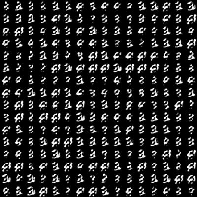
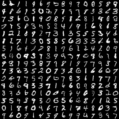
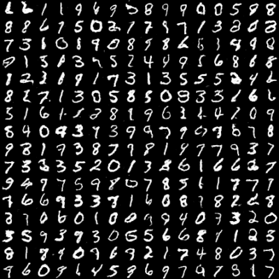
Let’s look at some of our Generator’s improved images in Figures 6-9.

In Figure 6, we can see that since the Generator just started training, the images produced are pretty much gibberish. In Figure 7, we can see a slight improvement in the images generated as they slowly take shape.

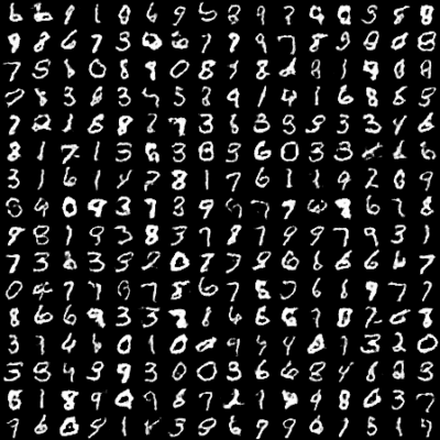
In Figures 8 and 9, we see complete Images being formed, which look like they have been plucked right out of the MNIST dataset, which means our Generator learned pretty well and ended up producing some really good images!

Summary

GANs have opened a whole new door for Machine Learning. We have consistently seen many new concepts produced by GANs and many old concepts being reproduced using GANs as their base. This simple yet ingenious concept is powerful enough to outperform most other algorithms in their respective fields.

In the training figures, we have seen that by the 20th epoch itself, our DCGAN became powerful enough to produce complete and distinguishable images. But I encourage you to use the coding skills you have learned here on various other tasks and datasets and see for yourself the magic of GANs.

Through this tutorial, I have tried to explain the basic essence of GANs and DCGANs using the MNIST dataset. I hope this tutorial helped you realize how epic GANs are!

Citation Information

Chakraborty, D. “Training a DCGAN in PyTorch,” PyImageSearch, 2021, https://pyimagesearch.com/2021/10/25/training-a-dcgan-in-pytorch/

@article{Chakraborty_2021_Training_DCGAN,
   author = {Devjyoti Chakraborty},
   title = {Training a {DCGAN} in {PyTorch}},
   journal = {PyImageSearch},
   year = {2021},
   note = {https://pyimagesearch.com/2021/10/25/training-a-dcgan-in-pytorch/},
}

To download the source code to this post (and be notified when future tutorials are published here on PyImageSearch), simply enter your email address in the form below!