Get Started: DCGAN for Fashion-MNIST

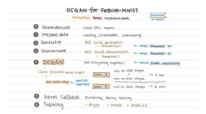
In this tutorial, we are implementing a Deep Convolutional GAN (DCGAN) with TensorFlow 2 / Keras, based on the paper, Unsupervised Representation Learning with Deep Convolutional Generative Adversarial Networks (Radford et al., 2016). This was one of the earliest GAN papers and is typically what you’d read to get started with learning GANs.

This is the second post of our GAN tutorial series:

1. Intro to Generative Adversarial Networks (GANs)
2. Get Started: DCGAN for Fashion-MNIST (this post)
3. GAN Training Challenges: DCGAN for Color Images

We will discuss these key topics in this post:

1. DCGAN architecture guidelines
2. Customized train_step() with Keras model.fit()
3. DCGAN implementation with TensorFlow 2 / Keras

Before we get started, are you familiar with how GANs work?

If not, be sure to look at my previous post, “Intro to GANs,” for a high-level intuition of how GANs work in general. Each GAN has at least one generator and one discriminator. While the generator and discriminator compete against each other, the generator gets better at generating images close to the distribution of the training data as it gets feedback from the discriminator.

To learn how to train a DCGAN using TensorFlow 2 / Keras to generate Fashion-MNIST like gray-scale images, just keep reading.

Architecture Guidelines

The DCGAN paper introduced a GAN architecture where the discriminator and generator are defined with convolutional neural networks (CNNs).

It provides several architecture guidelines to improve training stability (see Figure 1):

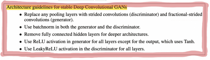
Let’s go through the guidelines above. For brevity, I will refer to the generator as G, and the discriminator as D.

Convolutions

• Strided convolutions: convolutional layer with a stride of 2, used for downsampling in D. See Figure 2 (left).
• Fractional-strided convolutions: Conv2DTranspose layer with a stride of 2 for upsampling in G. See Figure 2 (right).

• 

• 

Batch Normalization

The paper suggests using batch normalization (batchnorm) in both G and D to help stabilize GAN training. Batchnorm standardizes the input layer to have a zero mean and unit variance. It’s typically added after the hidden layer and before the activation layer. As we progress in the GAN series, you will learn better normalization techniques for GANs. For now, we will stay with the DCGAN paper recommendation of using batchnorm.

Activation

There are four commonly used activation functions in DCGAN generator and discriminator: sigmoid, tanh, ReLU, and leakyReLU as illustrated in Figure 3:

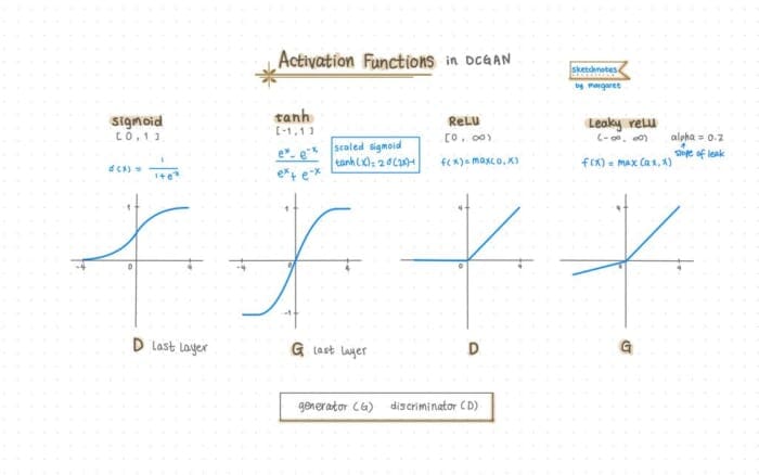
1. sigmoid: squashes the number to 0 (fake) and 1 (real). Since the DCGAN discriminator does binary classification, we use sigmoid in the last layer of D.
2. tanh (Hyperbolic Tangent): is also s-shaped like sigmoid; in fact, it’s a scaled sigmoid but centered at 0 and squashes the input value to [-1, 1]. As recommended by the paper, we use tanh in the last layer of G. This is why we need to preprocess our training images to the range of [-1, 1].
3. ReLU (Rectified Linear Activation): returns 0 when the input value is negative; otherwise, it returns the input value. The paper recommends ReLU activation for all layers in G except for the output layer, which uses tanh.
4. LeakyReLU: similar to ReLU except when the input value is negative, it uses a constant alpha to give it a very small slope. As suggested by the paper, we set the slope (alpha) as 0.2. We use LeakyReLU activation in D for all layers except for the last layer.

DCGAN Code in Keras

Now that we have a good understanding of the guidelines from the paper, let’s walk through the code to see how to implement DCGAN in TensorFlow 2 / Keras (see Figure 4).

Same as in the original vanilla GAN, we train two networks simultaneously: a generator and a discriminator. To create the DCGAN model, we first need to define the model architecture for the generator and discriminator with Keras Sequential API. Then we use Keras model subclassing to create the DCGAN.

Please follow the tutorial with this Colab notebook here.

Dependencies

Let’s first enable Colab GPU and import the libraries needed.

Enable Colab GPU

The code in this tutorial is in a Google Colab notebook, and it’s best to enable the free GPU offered by Colab. To enable GPU runtime in Colab, go to Edit → Notebook Settings or Runtime → change runtime type, and then select “GPU” from the Hardware Accelerator drop-down menu.

Imports

Colab should already have all the packages we need for this tutorial pre-installed. We will be writing the code in TensorFlow 2 / Keras and use matplotlib for visualization. We just need to import these libraries as follows:

import tensorflow as tf

from tensorflow import keras
from tensorflow.keras.datasets import fashion_mnist
from tensorflow.keras.models import Sequential
from tensorflow.keras import layers
from tensorflow.keras.models import Model
from tensorflow.keras.optimizers import Adam

from matplotlib import pyplot as plt

Data

The first step is to get data ready for training. For this post, we will train the DCGAN with the Fashion-MNIST data.

Data Loading

The Fashion-MNIST dataset has a train/test split. For training DCGAN, we don’t need such a data split. We can use only the training data or load both training/test datasets for training purposes.

For DCGAN with Fashion-MNIST, training with only the training dataset is sufficient:

(train_images, train_labels), (_, _) = tf.keras.datasets.fashion_mnist.load_data()

Take a look at the Fashion-MNIST training data shape with train_images.shape and notice the shape of (60000, 28, 28), meaning there are 60,000 training gray-scale images with the size of 28x28.

Data Visualization

I always like to visualize the training data to get an idea of what the images look like. Let’s look at one image to see what a Fashion-MNIST gray-scale 28x28x1 image looks like ​​(see Figure 5).

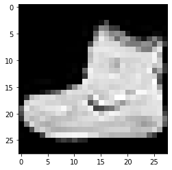
plt.figure()
plt.imshow(train_images[0], cmap='gray')
plt.show()

Data Preprocessing

The data loaded is in the shape of (60000, 28, 28) since it’s grayscale. So we need to add the 4th dimension for the channel as 1, and convert the data type (from NumPy array) to float32 as required for training in TensorFlow.

train_images = train_images.reshape(train_images.shape[0], 28, 28, 1).astype('float32')

We normalize the input image to the range of [-1, 1] because the generator’s final layer activation uses tanh as mentioned earlier.

train_images = (train_images - 127.5) / 127.5

The Generator Model

The generator’s job is to generate plausible images. Its objective is trying to fool the discriminator into thinking its generated images are real.

The generator takes random noise as an input and outputs an image that resembles the training images. Since we are generating a 28x28 gray-scale image here, the model architecture needs to make sure we arrive at a shape such that the generator output should be 28x28x1 (see Figure 6).

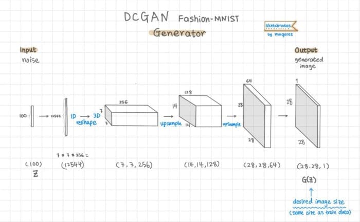
So to be able to create the image, the generator’s main tasks are:

• Convert the 1D random noise (latent vector) to 3D with the Reshape layer
• Upsample a few times with Keras Conv2DTranspose layer (fractional-strided convolution as referred to in the paper), to the output image size, in the case of Fashion-MNIST, a grayscale image in the shape of 28x28x1.

There are a few layers forming building blocks for G:

• Dense (fully connected) layer: only for reshaping and flatting the noise vector
• Conv2DTranspose: upsampling
• BatchNormalization: stabilize training; after the conv layer and before the activation function.
• Use ReLU activation in G for all layers except for the output, which uses tanh.

Let’s create a function for building the generator model architecture def build_generator().

Define a few parameters:

• latent dimension for the random noise
• weight initialization for the Con2DTranspose layer
• color channel of the images.

# latent dimension of the random noise
LATENT_DIM = 100
# weight initializer for G per DCGAN paper
WEIGHT_INIT = tf.keras.initializers.RandomNormal(mean=0.0, stddev=0.02)
# number of channels, 1 for gray scale and 3 for color images
CHANNELS = 1

Create a model with Keras Sequential API, which is the simplest way to create a model:

   model = Sequential(name='generator')

Then we create a Dense layer to prepare for reshaping to 3D, also make sure to define the input shape in this first layer of the model architecture. Add the BatchNormalization and ReLU layers:

   model.add(layers.Dense(7 * 7 * 256, input_dim=LATENT_DIM))
   model.add(layers.BatchNormalization())
   model.add(layers.ReLU())

Now we reshape the previous layer from 1D to 3D.

   model.add(layers.Reshape((7, 7, 256)))

Up sample twice with Conv2DTranspose with stride of 2 to get from 7x7 to 14x14 to 28x28. Add a BatchNormalization then a ReLU layer after each Conv2DTranspose layer.

   # upsample to 14x14: apply a transposed CONV => BN => RELU
   model.add(layers.Conv2DTranspose(128, (5, 5), strides=(2, 2),padding="same", kernel_initializer=WEIGHT_INIT))
   model.add(layers.BatchNormalization())
   model.add((layers.ReLU()))

   # upsample to 28x28: apply a transposed CONV => BN => RELU
   model.add(layers.Conv2DTranspose(64, (5, 5), strides=(2, 2),padding="same", kernel_initializer=WEIGHT_INIT))
   model.add(layers.BatchNormalization())
   model.add((layers.ReLU()))

And finally, we use a Conv2D layer with activation of tanh. Note CHANNELS was defined earlier as 1, which will make an image of 28x28x1, matching our gray-scale training image.

model.add(layers.Conv2D(CHANNELS, (5, 5), padding="same", activation="tanh"))

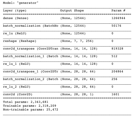
Take a look at the generator model architecture we just defined with generator.summary() to make sure that each layer is in the shape we want (see Figure 7):

The Discriminator Model

The discriminator is a simple binary classifier that tells whether an image is real or fake. Its objective is trying to classify the images correctly. There are a couple of differences between a discriminator and a regular classifier, though:

• We use LeakyReLU as the activation function per DCGAN paper.
• The discriminator has two groups of input images: the training dataset or real images labeled as 1, and the fake images created by the generator, labeled as 0.

Note: The discriminator network is typically smaller or simpler than the generator since the discriminator has a much easier job than the generator. If the discriminator is too strong, then the generator won’t improve well.

Here is what the discriminator architecture looks like (see Figure 8):

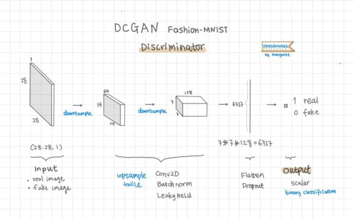
We will again create a function to build the discriminator model. The input to the discriminator is either the real images (training dataset) or the fake images generated by the generator, so the image size is 28x28x1 for Fashion-MNIST, which are passed in as argos into the function as width, height, and depth. The alpha is for LeakyReLU defining how much slope the leak is.

def build_discriminator(width, height, depth, alpha=0.2):

Use the Keras Sequential API to define the discriminator architecture.

   model = Sequential(name='discriminator')
   input_shape = (height, width, depth)

We use Conv2D, BatchNormalization, and LeakyReLU twice to downsample.

   # first set of CONV => BN => leaky ReLU layers
   model.add(layers.Conv2D(64, (5, 5), strides=(2, 2), padding="same",
       input_shape=input_shape))
   model.add(layers.BatchNormalization())
   model.add(layers.LeakyReLU(alpha=alpha))
 
   # second set of CONV => BN => leacy ReLU layers
   model.add(layers.Conv2D(128, (5, 5), strides=(2, 2), padding="same"))
   model.add(layers.BatchNormalization())
   model.add(layers.LeakyReLU(alpha=alpha))

Flatten and apply dropout:

   model.add(layers.Flatten())
   model.add(layers.Dropout(0.3))

Then in the last layer, we use the sigmoid activation function to output a single value for binary classification.

   model.add(layers.Dense(1, activation="sigmoid"))

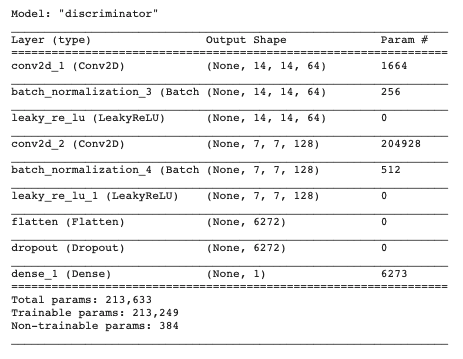
Call model.summary() to see the discriminator architecture we just defined (see Figure 9):

Loss Function

Let’s talk about the loss function before moving on to creating the DCGAN model.

Calculating the loss is at the heart of the DCGAN (or any GAN) training. For DCGAN, we will implement the modified minimax loss, which uses the binary cross-entropy (BCE) loss function. As we progress in the GANs series, you will learn other loss functions in different GAN variants.

There are 2 losses that we will need to calculate: one for the discriminator loss and the other one for the generator loss.

The Discriminator Loss

Since there are two groups of images being fed into the discriminator (real images and fake images), we will calculate the loss on each and combine them for the discriminator loss.

Total D loss = loss_from_real_images + loss_from_fake_images

The Generator Loss

For the generator loss, rather than training G to minimize log(1 − D(G(z))) – the probability that D classifiers fake images as fake (0), we can train G to maximize log D(G(z)) – the probability that D incorrectly classifies the fake images as real (1). So this is the modified minimax loss.

The DCGAN Model: Override train_step

We have defined the generator and discriminator architecture and understand how the loss function works. We are ready to put D and G together to create the DCGAN model by subclassing keras.Model and overriding train_step() to train the discriminator and the generator. Here is the documentation on how to write the low-level code to customize model.fit(). The advantage of this approach is that you can still use GradientTape for the custom training loop while still benefiting from the convenient features of fit() (e.g., callbacks, and built-in distribution support, etc.).

So we subclass keras.Model to create the DCGAN class – class DCGAN(keras.Model):

Please refer to the Colab notebook here for details of the DCGAN class, and here I’m only focusing on the explanation of how to override train_step() for training D and G.

In train_step(), we first create the random noise that is the input for the generator:

batch_size = tf.shape(real_images)[0]
noise = tf.random.normal(shape=(batch_size, self.latent_dim))

Then we train the discriminator with both real images (labeled as 1) and fake images (labeled as 0).

with tf.GradientTape() as tape:
    # Compute discriminator loss on real images
    pred_real = self.discriminator(real_images, training=True)
    d_loss_real = self.loss_fn(tf.ones((batch_size, 1)), pred_real)

    # Compute discriminator loss on fake images
    fake_images = self.generator(noise)
    pred_fake = self.discriminator(fake_images, training=True)
    d_loss_fake = self.loss_fn(tf.zeros((batch_size, 1)), pred_fake)

    # total discriminator loss
    d_loss = (d_loss_real + d_loss_fake)/2
# Compute discriminator gradients
grads = tape.gradient(d_loss, self.discriminator.trainable_variables)
# Update discriminator weights
self.d_optimizer.apply_gradients(zip(grads, self.discriminator.trainable_variables))

We train the generator while not updating the weights of the discriminator.

misleading_labels = tf.ones((batch_size, 1)) 

with tf.GradientTape() as tape:
    fake_images = self.generator(noise, training=True)
    pred_fake = self.discriminator(fake_images, training=True)
    g_loss = self.loss_fn(misleading_labels, pred_fake)
# Compute generator gradients
grads = tape.gradient(g_loss, self.generator.trainable_variables)
# Update generator weights
self.g_optimizer.apply_gradients(zip(grads, self.generator.trainable_variables))

self.d_loss_metric.update_state(d_loss)
self.g_loss_metric.update_state(g_loss)

Monitoring and Visualization During Training

We will override Keras Callback() to monitor:

1. Discriminator loss
2. Generator loss
3. Images that get generated during training

For image classification, for example, the losses can help us understand how the model is performing. For GANs, D losses and G losses indicate how each model is performing individually and may or may not be an accurate measure of how the GAN model is doing in general. We will discuss this further in the next post of “GAN training challenges.”

For GAN evaluation, it’s important that we visually inspect the images that get generated during training. We will learn other evaluation methods in future posts.

Compile and Train the Model

Now we can finally put together the DCGAN model!

dcgan = DCGAN(discriminator=discriminator, generator=generator, latent_dim=LATENT_DIM)

As suggested by the DCGAN paper, we use the Adam optimizer with a learning rate of 0.0002 for both the generator and discriminator. As mentioned earlier, we use the Binary Cross-Entropy loss function for both D and G.

LR = 0.0002 # learning rate

dcgan.compile(
   d_optimizer=keras.optimizers.Adam(learning_rate=LR, beta_1 = 0.5),
   g_optimizer=keras.optimizers.Adam(learning_rate=LR, beta_1 = 0.5),
   loss_fn=keras.losses.BinaryCrossentropy(),
)

We are ready to train the DCGAN model by simply calling model.fit!

NUM_EPOCHS = 50 # number of epochs
dcgan.fit(train_images, epochs=NUM_EPOCHS, 
callbacks=[GANMonitor(num_img=16, latent_dim=LATENT_DIM)])

Train for 50 epochs, and each epoch only takes about 25 seconds with GPU in a Colab notebook.

During training, we can visually inspect the generated images to make sure the generator is generating images of good quality.

Looking at the Images generated during training at the 1st epoch, 25th epoch, and 50th epoch in Figure 10, we see that the generator is getting better at generating Fashion-MNIST look-alike images.

Summary

In this post, we covered the DCGAN architecture guidelines on how to train a stable DCGAN. Along with a Colab notebook, we walked through the DCGAN code implementation with gray-scale Fashion-MNIST images in TensorFlow 2 / Keras. I discussed how to customize train_step with Keras Model subclassing and then calling Keras model.fit() for training. In the next post, I will demonstrate the challenges of GAN training by implementing a DCGAN trained with fashion color images.

Citation Information

Maynard-Reid, M. “Get Started: DCGAN for Fashion-MNIST,” PyImageSearch, 2021, https://pyimagesearch.com/2021/11/11/get-started-dcgan-for-fashion-mnist/

@article{Maynard-Reid_2021_DCGAN_MNIST,
  author = {Margaret Maynard-Reid},
  title = {Get Started: {DCGAN} for Fashion-{MNIST}},
  journal = {PyImageSearch},
  year = {2021},
  note = {https://pyimagesearch.com/2021/11/11/get-started-dcgan-for-fashion-mnist/},
}

To download the source code to this post (and be notified when future tutorials are published here on PyImageSearch), simply enter your email address in the form below!