In this tutorial, you will learn how to perform automatic color correction with OpenCV using a color matching/balancing card.
Last week we discovered how to perform histogram matching. Using histogram matching, we can take the color distribution of one image and match it to another.
A practical, real-world application of color matching is to perform basic color correction through color constancy. The goal of color constancy is to perceive the colors of objects correctly regardless of differences in light sources, illumination, etc. (which, as you can imagine, is easier said than done).
Photographers and computer vision practitioners can help obtain color constancy by using color correction cards, like this one:
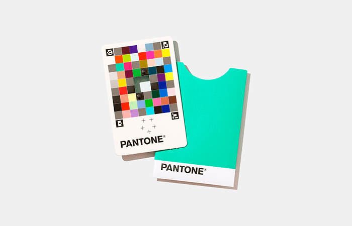
Using a color correction/color constancy card, we can:
- Detect the color correction card in an input image
- Compute the histogram of the card, which contains gradated colors of varying colors, hues, shades, blacks, whites, and grays
- Apply histogram matching from the color card to another image, thereby attempting to achieve color constancy
In this tutorial, we’ll build a color correction system with OpenCV by putting together all the pieces we’ve learned from previous tutorials on:
- Detecting ArUco markers with OpenCV and Python
- OpenCV Histogram Equalization and Adaptive Histogram Equalization (CLAHE)
- Histogram matching with OpenCV, scikit-image, and Python
By the end of the guide, you will understand the fundamentals of how color correction cards can be used in conjunction with histogram matching to build a basic color corrector, regardless of the illumination conditions under which an image was captured.
To learn how to perform basic color correction with OpenCV, just keep reading.
Automatic color correction with OpenCV and Python
In the first part of this tutorial, we’ll discuss what color correction and color constancy are, including how OpenCV can facilitate automatic color correction.
We’ll then configure our development environment for this project and review our project directory structure.
With our development environment ready, we’ll implement a Python script that leverages OpenCV to perform color correction.
We’ll wrap up this tutorial with a discussion of our results.
What is automatic color correction?
The human visual system is impacted significantly by illumination and light sources. Color constancy refers to the study of how humans perceive color.
For example, take a look at the following image from the Wikipedia article on color constancy:
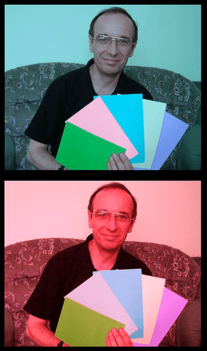
Looking at this card, it seems that the pink shade (second from the left) is substantially stronger than the pink shade on the bottom — but as it turns out, they are the same color!
Both these cards have the same RGB values. However, our human color perception system is affected by the color cast of the rest of the photo (i.e., applying a warm red filter on top of it).
That creates a bit of a problem if we seek to normalize our image processing environment. As I stated in my previous tutorial on Detecting low contrast images:
It’s far easier to write code for images captured in controlled conditions than in dynamic conditions with no guarantees.
If we can control our image capturing environment as much as possible, the easier it will be to write code to analyze and process these images captured from the controlled environment.
Think about it this way . . . suppose we can safely assume the lighting conditions of an environment. In that case, we can ditch expensive computer vision/deep learning algorithms, which help us obtain desirable results in non-ideal conditions. We instead leverage basic image processing routines, allowing us to hardcode parameters, including Gaussian blur sizes, Canny edge detection thresholds, etc.
Essentially, with controlled environments, we can get away with basic image processing algorithms that are far easier to implement. The catch is that we need safe assumptions on our lighting conditions. Color correction and white balancing help us achieve that.
One way we can help control our environment, even if lighting conditions change a bit, is to apply color correction.
Color checking cards are a favorite tool of photographers:
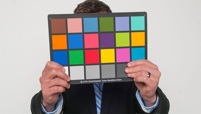
Photographers place these cards into scenes they are capturing. They then snap photos, adjusting their lighting (while still keeping the card in view of the camera), and then continue shooting until they are done.
After shooting, they go back to their computer, transfer the photos onto their system, and use a tool such as Adobe Lightroom to achieve color consistency across the entire shoot (here’s a tutorial on doing that process if you are interested).
Of course, as computer vision practitioners, we do not have the luxury of using Adobe Lightroom, nor would we want to start/stop our pipeline by manually adjusting color balancing — defeating the entire purpose of using software to automate real-world processes.
Instead, we can leverage these same color correction cards, and along with a bit of histogram matching, we can build a system capable of performing color correction.
In the rest of this guide, you will utilize histogram matching and a color correction card (from Pantone) to perform basic color correction.
Pantone’s color correction card

For this tutorial, we’ll be using Pantone’s Color Match card.
This card is similar to a color correction card that photographers use but is instead used by Pantone to help their consumers match perceived colors in a scene to a shade of paint (most similar to that color) that Pantone sells.
The general idea is that:
- You place the color correction card over the shade you want to match
- You open Pantone’s smartphone app on your phone
- You snap a photo of the card
- The app automatically detects the card, performs color matching, and then returns the most similar shades that Pantone sells
For our purposes, we’ll be using the card strictly for color correction (but you could easily extend it as you see fit).
Configuring your development environment
To learn how to perform automatic color correction, you need to have both OpenCV and scikit-image installed:
Both are pip-installable using the following commands:
$ pip install opencv-contrib-python
$ pip install scikit-image==0.18.1
If you need help configuring your development environment for OpenCV, I highly recommend that you read my pip install OpenCV guide — it will have you up and running in a matter of minutes.
Having problems configuring your development environment?
All that said, are you:
- Short on time?
- Learning on your employer’s administratively locked system?
- Wanting to skip the hassle of fighting with the command line, package managers, and virtual environments?
- Ready to run the code right now on your Windows, macOS, or Linux systems?
Then join PyImageSearch Plus today!
Gain access to Jupyter Notebooks for this tutorial and other PyImageSearch guides that are pre-configured to run on Google Colab’s ecosystem right in your web browser! No installation required.
And best of all, these Jupyter Notebooks will run on Windows, macOS, and Linux!
Project structure
While color matching and color correction may seem like a complicated process, as we’ll find out, we’ll be able to complete the entire project in just under 100 lines of code (including comments).
But before we start coding, let’s first review our project directory structure.
Start by accessing the “Downloads” section of this tutorial to retrieve the source code and example images — then take a look at the folder:
$ tree . --dirsfirst
.
├── examples
│   ├── 01.jpg
│   ├── 02.jpg
│   └── 03.jpg
├── color_correction.py
└── reference.jpg

1 directory, 5 files
We have a single Python script to review today, color_correction.py. This script will:
- Load our
reference.pngimage (which contains our Pantone color correction card) - Load one of the images in the
examplesdirectory (which we’ll color correct to match that ofreference.png) - Detect the color matching card via ArUco marker detection in both the reference and input image
- Apply histogram matching to round out the color correction process
Let’s get to work!
Implementing automatic color correction with OpenCV
We are now ready to implement color correction with OpenCV and Python.
Open the color_correction.py file in your project directory structure, and let’s get to work:
# import the necessary packages
from imutils.perspective import four_point_transform
from skimage import exposure
import numpy as np
import argparse
import imutils
import cv2
import sys
We start on Lines 2-8, importing our required Python packages. The notable ones include:
four_point_transform: Applies a perspective transform to obtain a top-down, bird’s-eye view of the input color matching card. See the following tutorial for an example of using this function.exposure: Contains the histogram matching function from scikit-image.imutils: My set of convenience functions for performing image processing with OpenCV.cv2: Our OpenCV bindings.
With our imports taken care of, we can move on to defining the find_color_card function, the method responsible for locating the Pantone color matching card in an input image:
def find_color_card(image):
	# load the ArUCo dictionary, grab the ArUCo parameters, and
	# detect the markers in the input image
	arucoDict = cv2.aruco.Dictionary_get(cv2.aruco.DICT_ARUCO_ORIGINAL)
	arucoParams = cv2.aruco.DetectorParameters_create()
	(corners, ids, rejected) = cv2.aruco.detectMarkers(image,
		arucoDict, parameters=arucoParams)
Our find_color_card function requires only a single parameter, image, which is the image that (presumably) contains our color matching card.
From there, Lines 13-16 perform ArUco marker detection to find the four ArUco markers on the color matching card itself.
Next, let’s order the four ArUco markers in top-left, top-right, bottom-right, and bottom-left order (the required order for applying a top-down perspective transform):
	# try to extract the coordinates of the color correction card
	try:
		# otherwise, we've found the four ArUco markers, so we can
		# continue by flattening the ArUco IDs list
		ids = ids.flatten()

		# extract the top-left marker
		i = np.squeeze(np.where(ids == 923))
		topLeft = np.squeeze(corners[i])[0]

		# extract the top-right marker
		i = np.squeeze(np.where(ids == 1001))
		topRight = np.squeeze(corners[i])[1]

		# extract the bottom-right marker
		i = np.squeeze(np.where(ids == 241))
		bottomRight = np.squeeze(corners[i])[2]

		# extract the bottom-left marker
		i = np.squeeze(np.where(ids == 1007))
		bottomLeft = np.squeeze(corners[i])[3]

	# we could not find color correction card, so gracefully return
	except:
		return None
First, we wrap this entire code block in a try/except block. We do this just in case all four markers cannot be detected using np.where calls. If only a single np.where call fails, Python will throw an error.
Our try/except block will catch the error and return None, implying that the color correction card could not be found.
Otherwise, Lines 25-38 extract each of the individual ArUco markers in top-left, top-right, bottom-right, and bottom-left order.
Note: You may be wondering how I knew the IDs for each of the markers was going to be 923, 1001, 241, and 1007? That is addressed in my previous set of tutorials on ArUco marker detection. Be sure you give that tutorial a read if you haven’t read it yet.
Provided we found all four ArUco markers, and we can now apply the perspective transform:
	# build our list of reference points and apply a perspective
	# transform to obtain a top-down, bird’s-eye view of the color
	# matching card
	cardCoords = np.array([topLeft, topRight,
		bottomRight, bottomLeft])
	card = four_point_transform(image, cardCoords)

	# return the color matching card to the calling function
	return card
Lines 47-49 build a NumPy array from our ArUco marker coordinates and then apply the four_point_transform function to obtain a top-down, bird’s-eye view of the color correction card.
This top-down view of the card is returned to the calling function.
With our find_color_card function implemented, let’s move on to parsing command line arguments:
# construct the argument parser and parse the arguments
ap = argparse.ArgumentParser()
ap.add_argument("-r", "--reference", required=True,
	help="path to the input reference image")
ap.add_argument("-i", "--input", required=True,
	help="path to the input image to apply color correction to")
args = vars(ap.parse_args())
To perform color matching, we need two images:
- The path to the
--referenceimage contains the input scene in the “ideal” conditions to which we want to correct any input image. - The path to the
--inputimage, which we assume has a different color distribution, presumably due to changes in lighting conditions.
Our goal is to take the --input image and perform color matching such that its distribution matches that of the --reference image.
But before we can do that, we need to load the reference and source images from disk:
# load the reference image and input images from disk
print("[INFO] loading images...")
ref = cv2.imread(args["reference"])
image = cv2.imread(args["input"])

# resize the reference and input images
ref = imutils.resize(ref, width=600)
image = imutils.resize(image, width=600)

# display the reference and input images to our screen
cv2.imshow("Reference", ref)
cv2.imshow("Input", image)
Lines 64 and 65 load our input images from disk, while Lines 68 and 69 preprocess them by resizing to a width of 600 pixels (to process the images faster).
Lines 72 and 73 then display the original ref and image to our screen.
With our images loaded, let’s now apply the find_color_card function to both images:
# find the color matching card in each image
print("[INFO] finding color matching cards...")
refCard = find_color_card(ref)
imageCard = find_color_card(image)

# if the color matching card is not found in either the reference
# image or the input image, gracefully exit
if refCard is None or imageCard is None:
	print("[INFO] could not find color matching card in both images")
	sys.exit(0)
Lines 77 and 78 attempt to locate the color matching card in both the ref and image.
If we cannot find the color matching card in either image, we gracefully exit the script (Lines 82-84).
Otherwise, we can safely assume we found the color matching card, so let’s apply color correction:
# show the color matching card in the reference image and input image,
# respectively
cv2.imshow("Reference Color Card", refCard)
cv2.imshow("Input Color Card", imageCard)

# apply histogram matching from the color matching card in the
# reference image to the color matching card in the input image
print("[INFO] matching images...")
imageCard = exposure.match_histograms(imageCard, refCard,
	multichannel=True)

# show our input color matching card after histogram matching
cv2.imshow("Input Color Card After Matching", imageCard)
cv2.waitKey(0)
Lines 88 and 89 display our refCard and imageCard to our screen.
We then apply the match_histograms function to transfer the color distribution from the refCard to the imageCard.
Finally, the output imageCard, after histogram matching, is displayed on our screen. This new imageCard now contains the color corrected version of the original imageCard.
Automatic color correction results
We are now ready to perform automatic color correction with OpenCV!
Be sure to access the “Downloads” section of this tutorial to retrieve the source code and example images.
From there, you can open a shell and execute the following command:
$ python color_correction.py --reference reference.jpg \
	--input examples/01.jpg
[INFO] loading images...
[INFO] finding color matching cards...
[INFO] matching images...
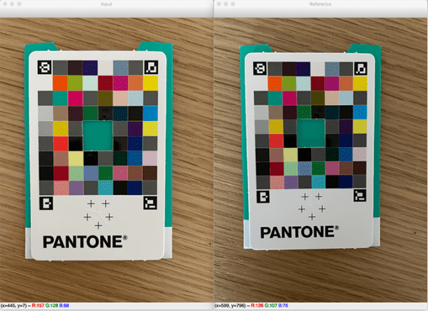
On the left, we have our reference image. Notice how we placed the color correction card over a shade of teal. Our goal here is to ensure that shade of teal is consistent across all input images, regardless of how lighting conditions change.
Now, examine the photo on the right. This is our example input image. You can see that due to lighting conditions, the shade of teal is slightly brighter than the shade of teal in the reference image.
How can we correct this appearance?
The answer is to apply color correction:
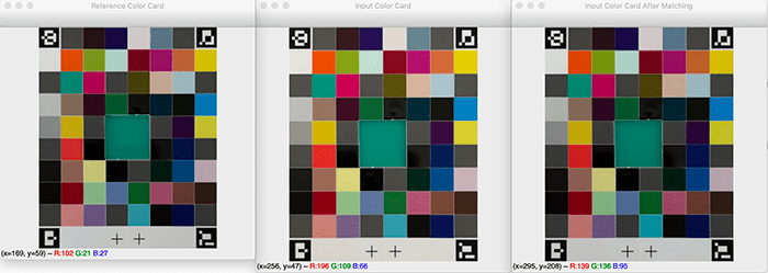
On the left, we have detected the color card in the reference image. The middle shows the color card from the input image. And finally, the right displays the input color card after color matching.
Notice how the shade of teal on the right more closely resembles the shade of teal in the input reference image (i.e., the shade of teal on the right is darker than the one in the middle).
Let’s try another image:
$ python color_correction.py --reference reference.jpg \
	--input examples/02.jpg
[INFO] loading images...
[INFO] finding color matching cards...
[INFO] matching images...

Again, we start with our reference image (left) and our input image (right), to which we seek to apply color correction.
Below is our output after applying color matching:
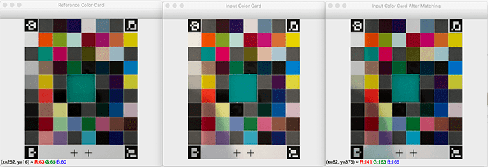
The left contains the color matching card from the reference image, while the middle displays the color matching card from the input image (02.jpg). You can see that the shade of teal in the middle image is significantly brighter than the shade of teal on the left.
By applying color matching and correction, we can correct this disparity (right). Notice how the shades of teal on the left and right more similarly match each other.
Here is one final example:
$ python color_correction.py --reference reference.jpg \
	--input examples/03.jpg
[INFO] loading images...
[INFO] finding color matching cards...
[INFO] matching images...
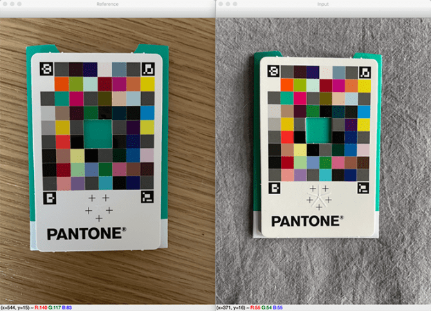
Here, the lighting conditions are significantly different from the previous two. The image on the left is our reference image (captured in my office), while the image on the right is the input image (captured in my bedroom).
Due to the windows in the bedroom and how the sun was entering the windows that day, there is significant shadowing on the right side of the color matching card, thereby making this more of a challenge (and demonstrating some of the limitations of this basic color correction method).
Below is the output of applying color correction via histogram matching:
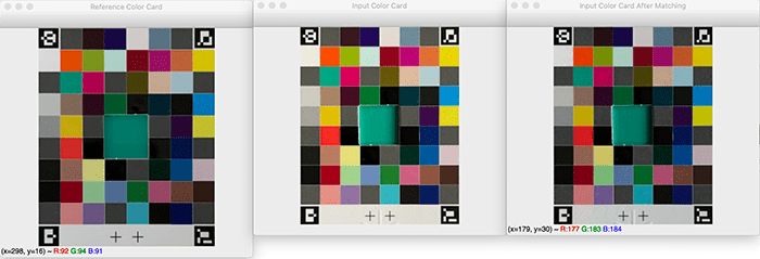
The left image is the color matching card from our reference image. We then have the detected color correction card from our input image (03.jpg).
Applying histogram matching yields the right image. While we still have shadowing, we can see that the brighter teal color from the middle has been corrected to more similarly match the original darker teal color from the reference image.
What's next? We recommend PyImageSearch University.
86+ total classes • 115+ hours hours of on-demand code walkthrough videos • Last updated: April 2026
★★★★★ 4.84 (128 Ratings) • 16,000+ Students Enrolled
I strongly believe that if you had the right teacher you could master computer vision and deep learning.
Do you think learning computer vision and deep learning has to be time-consuming, overwhelming, and complicated? Or has to involve complex mathematics and equations? Or requires a degree in computer science?
That’s not the case.
All you need to master computer vision and deep learning is for someone to explain things to you in simple, intuitive terms. And that’s exactly what I do. My mission is to change education and how complex Artificial Intelligence topics are taught.
If you're serious about learning computer vision, your next stop should be PyImageSearch University, the most comprehensive computer vision, deep learning, and OpenCV course online today. Here you’ll learn how to successfully and confidently apply computer vision to your work, research, and projects. Join me in computer vision mastery.
Inside PyImageSearch University you'll find:
- ✓ 86+ courses on essential computer vision, deep learning, and OpenCV topics
- ✓ 86 Certificates of Completion
- ✓ 115+ hours hours of on-demand video
- ✓ Brand new courses released regularly, ensuring you can keep up with state-of-the-art techniques
- ✓ Pre-configured Jupyter Notebooks in Google Colab
- ✓ Run all code examples in your web browser — works on Windows, macOS, and Linux (no dev environment configuration required!)
- ✓ Access to centralized code repos for all 540+ tutorials on PyImageSearch
- ✓ Easy one-click downloads for code, datasets, pre-trained models, etc.
- ✓ Access on mobile, laptop, desktop, etc.
Summary
In this tutorial, you learned how to perform basic color correction using OpenCV and Python.
We achieved this goal by:
- Placing a color correction card in the view of our camera
- Snapping a photo of the scene
- Detecting the color correction card with ArUco marker detection
- Applying histogram matching to transfer the color distribution of the card to another image
Taken together, we can think of this process as a color correction procedure (albeit quite basic).
Achieving pure color constancy, especially without markers/color correction cards, is still an active research area and will likely continue for many years to come. But in the meantime, we can leverage histogram matching and color matching cards to get us moving in the right direction.
To download the source code to this post (and be notified when future tutorials are published here on PyImageSearch), simply enter your email address in the form below!

Download the Source Code and FREE 17-page Resource Guide
Enter your email address below to get a .zip of the code and a FREE 17-page Resource Guide on Computer Vision, OpenCV, and Deep Learning. Inside you'll find my hand-picked tutorials, books, courses, and libraries to help you master CV and DL!


Comment section
Hey, Adrian Rosebrock here, author and creator of PyImageSearch. While I love hearing from readers, a couple years ago I made the tough decision to no longer offer 1:1 help over blog post comments.
At the time I was receiving 200+ emails per day and another 100+ blog post comments. I simply did not have the time to moderate and respond to them all, and the sheer volume of requests was taking a toll on me.
Instead, my goal is to do the most good for the computer vision, deep learning, and OpenCV community at large by focusing my time on authoring high-quality blog posts, tutorials, and books/courses.
If you need help learning computer vision and deep learning, I suggest you refer to my full catalog of books and courses — they have helped tens of thousands of developers, students, and researchers just like yourself learn Computer Vision, Deep Learning, and OpenCV.
Click here to browse my full catalog.