In this tutorial, you will learn to perform both histogram equalization and adaptive histogram equalization with OpenCV.

Histogram equalization is a basic image processing technique that adjusts the global contrast of an image by updating the image histogram’s pixel intensity distribution. Doing so enables areas of low contrast to obtain higher contrast in the output image.
Essentially, histogram equalization works by:
- Computing a histogram of image pixel intensities
- Evenly spreading out and distributing the most frequent pixel values (i.e., the ones with the largest counts in the histogram)
- Giving a linear trend to the cumulative distribution function (CDF)
The result of applying histogram equalization is an image with higher global contrast.
We can further improve histogram equalization by applying an algorithm called Contrast Limited Adaptive Histogram Equalization (CLAHE), resulting in higher quality output images.
Other than photographers using histogram equalization to correct under/over-exposed images, the most widely used histogram equalization application can be found in the medical field.
You’ll typically see histogram equalization applied to X-ray scans and CT scans to improve the radiograph’s contrast. Doing so helps doctors and radiologists better interpret the scans and make an accurate diagnosis.
By the end of this tutorial, you will be able to successfully apply both basic histogram equalization and adaptive histogram equalization to images with OpenCV.
To learn to use histogram equalization and adaptive histogram equalization with OpenCV, just keep reading.
OpenCV Histogram Equalization and Adaptive Histogram Equalization (CLAHE)
In the first part of this tutorial, we’ll discuss what histogram equalization is and how we can apply histogram equalization with OpenCV.
From there, we’ll configure our development environment and then review the project directory structure for this guide.
We’ll then implement two Python scripts:
simple_equalization.py: Performs basic histogram equalization using OpenCV’scv2.equalizeHistfunction.adaptive_equalization.py: Uses OpenCV’scv2.createCLAHEmethod to perform adaptive histogram equalization.
We’ll wrap up this guide with a discussion of our results.
What is histogram equalization?
Histogram equalization is a basic image processing technique that can improve an image’s overall contrast.
Applying histogram equalization starts by computing the histogram of pixel intensities in an input grayscale/single-channel image:
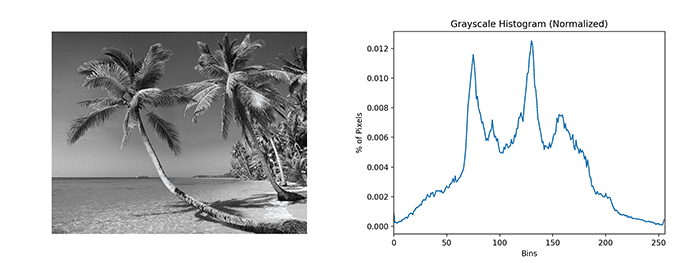
Notice how our histogram has numerous peaks, indicating there are a good number of pixels binned to those respective buckets. With histogram equalization, our goal is to spread these pixels to buckets that don’t have as many pixels binned to them.
Mathematically, what this means is that we’re attempting to apply a linear trend to our cumulative distribution function (CDF):

The before and after histogram equalization application can be seen in Figure 3:

Notice how the input image’s contrast has improved significantly but at the expense of also boosting the contrast of the noise in the input image.
That raises the question:
Is it possible to improve image contrast without also boosting noise at the same time?
The answer is “Yes,” you just need to apply adaptive histogram equalization.
With adaptive histogram equalization, we divide an input image into an M x N grid. We then apply equalization to each cell in the grid, resulting in a higher quality output image:

The downside is that adaptive histogram equalization is by definition more computationally complex (but given modern hardware, both implementations are still quite speedy).
How can we use OpenCV for histogram equalization?
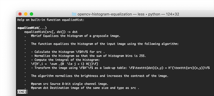
cv2.equalizeHist and cv2.createCLAHE.OpenCV includes implementations of both basic histogram equalization and adaptive histogram equalization through the following two functions:
cv2.equalizeHistcv2.createCLAHE
Applying the cv2.equalizeHist function is as simple as converting an image to grayscale and then calling cv2.equalizeHist on it:
gray = cv2.cvtColor(image, cv2.COLOR_BGR2GRAY)
equalized = cv2.equalizeHist(gray)
Performing adaptive histogram equalization requires that we:
- Convert the input image to grayscale/extract a single channel from it
- Instantiate the CLAHE algorithm using
cv2.createCLAHE - Call the
.applymethod on the CLAHE object to apply histogram equalization
It’s a lot easier than it sounds, requiring only a few lines of code:
gray = cv2.cvtColor(image, cv2.COLOR_BGR2GRAY)
clahe = cv2.createCLAHE(clipLimit=2.0, tileGridSize=(8, 8))
equalized = clahe.apply(gray)
Notice that we supply two parameters to cv2.createCLAHE:
clipLimit: This is the threshold for contrast limitingtileGridSize: Divides the input image into M x N tiles and then applies histogram equalization to each local tile
You will get practice using both cv2.equalizeHist and cv2.createCLAHE in the remainder of this guide.
Configuring your development environment
To learn how to apply histogram equalization with OpenCV, you need to have the OpenCV library installed.
Luckily, OpenCV is pip-installable:
$ pip install opencv-contrib-python
If you need help configuring your development environment for OpenCV, I highly recommend that you read my pip install OpenCV guide — it will have you up and running in a matter of minutes.
Having problems configuring your development environment?
All that said, are you:
- Short on time?
- Learning on your employer’s administratively locked system?
- Wanting to skip the hassle of fighting with the command line, package managers, and virtual environments?
- Ready to run the code right now on your Windows, macOS, or Linux system?
Then join PyImageSearch Plus today!
Gain access to Jupyter Notebooks for this tutorial and other PyImageSearch guides that are pre-configured to run on Google Colab’s ecosystem right in your web browser! No installation required.
And best of all, these Jupyter Notebooks will run on Windows, macOS, and Linux!
Project structure
Before we implement histogram equalization with OpenCV, let’s start by reviewing our project directory structure.
Be sure to access the “Downloads” section of this tutorial to retrieve the source code and example images.
From there, inspect the project directory structure:
$ tree . --dirsfirst
.
├── images
│   ├── boston.png
│   ├── dog.png
│   └── moon.png
├── adaptive_equalization.py
└── simple_equalization.py

1 directory, 5 files
We have two Python scripts that we’ll be reviewing today:
simple_equalization.py: Applies basic histogram equalization with OpenCV.adaptive_equalization.py: Uses the CLAHE algorithm to perform adaptive histogram equalization.
Our images directory contains example images to which we will apply histogram equalization.
Implementing standard histogram equalization with OpenCV
With our project directory structure reviewed, let’s move on to implementing basic histogram equalization with OpenCV.
Open the simple_equalization.py file in your project folder, and let’s get to work:
# import the necessary packages
import argparse
import cv2

# construct the argument parser and parse the arguments
ap = argparse.ArgumentParser()
ap.add_argument("-i", "--image", type=str, required=True,
	help="path to the input image")
args = vars(ap.parse_args())
Lines 2 and 3 import our required Python packages while Lines 6-9 parse our command line arguments.
We only need a single argument here, --image, which is the path to our input image on disk, where we wish to apply the histogram equalization.
With the command line arguments parsed, we can move on to the next step:
# load the input image from disk and convert it to grayscale
print("[INFO] loading input image...")
image = cv2.imread(args["image"])
gray = cv2.cvtColor(image, cv2.COLOR_BGR2GRAY)

# apply histogram equalization
print("[INFO] performing histogram equalization...")
equalized = cv2.equalizeHist(gray)
Line 13 loads our image from disk, while Line 14 converts our image from RGB to grayscale.
Line 18 performs basic histogram equalization using the cv2.equalizeHist function. The only required argument we must pass in is the grayscale/single-channel image.
Note: When performing histogram equalization with OpenCV, we must supply a grayscale/single-channel image. If we try to pass in a multi-channel image, OpenCV will throw an error. To perform histogram equalization on a multi-channel image, you would need to (1) split the image into its respective channels, (2) equalize each channel, and (3) merge the channels back together.
The final step is to show our output images:
# show the original grayscale image and equalized image
cv2.imshow("Input", gray)
cv2.imshow("Histogram Equalization", equalized)
cv2.waitKey(0)
Here, we are displaying our input gray image along with the histogram equalized image.
OpenCV histogram equalization results
We are now ready to apply basic histogram equalization with OpenCV!
Be sure to access the “Downloads” section of this tutorial to retrieve the source code and example images.
From there, open a terminal and execute the following command:
$ python simple_equalization.py --image images/moon.png
[INFO] loading input image...
[INFO] performing histogram equalization...
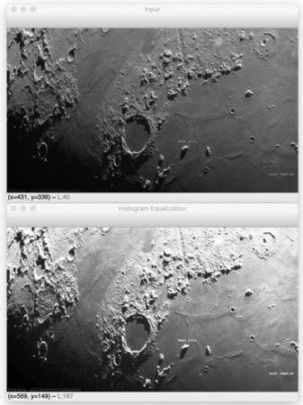
On the top, we have the original input image of the moon. The bottom shows the output after applying histogram equalization. Notice that we have boosted the image’s global contrast.
Let’s try a different image, this one of an under-exposed photograph:
$ python simple_equalization.py --image images/dog.png
[INFO] loading input image...
[INFO] performing histogram equalization...
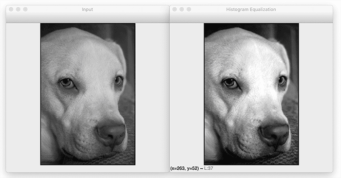
The dog (left) appears washed out due to underexposure. By applying histogram equalization (right), we correct this effect and improve the dog’s contrast.
The following image highlights one of the limitations of global contrast adjustment via histogram equalization:
$ python simple_equalization.py --image images/boston.png
[INFO] loading input image...
[INFO] performing histogram equalization...
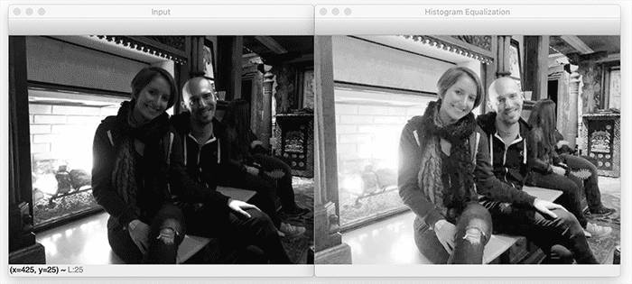
The image on the left shows my wife and me in Boston over the Christmas holiday a few years ago. Due to the auto-adjustment on the camera, our faces are quite dark, and it’s hard to see us.
By applying histogram equalization (right), we can see that not only are our faces visible, but we can see another couple sitting behind us! Without histogram equalization, you may have missed the other couple.
However, our output is not entirely desirable. To start, the fire in the fireplace is totally washed out. And if you study our faces, particularly mine, you’ll see that portions of my forehead are now totally washed out.
To improve our results, we need to apply adaptive histogram equalization.
Implementing adaptive histogram equalization with OpenCV
At this point, we’ve seen some of the limitations of basic histogram equalization.
While a bit more computationally expensive, adaptive histogram equalization can yield better results than simple histogram equalization. But don’t take my word for it — you should see the results for yourself.
Open the adaptive_equalization.py file in your project directory structure and insert the following code:
# import the necessary packages
import argparse
import cv2

# construct the argument parser and parse the arguments
ap = argparse.ArgumentParser()
ap.add_argument("-i", "--image", type=str, required=True,
	help="path to the input image")
ap.add_argument("-c", "--clip", type=float, default=2.0,
	help="threshold for contrast limiting")
ap.add_argument("-t", "--tile", type=int, default=8,
	help="tile grid size -- divides image into tile x time cells")
args = vars(ap.parse_args())
We only need two imports here, argparse for command line arguments and cv2 for our OpenCV bindings.
We then have three command line arguments, one of which is required, the second two optional (but useful to tune and play with when experimenting with CLAHE):
--image: The path to our input image on disk, where we wish to apply histogram equalization.--clip: The threshold for contrast limiting. You’ll typically want to leave this value in the range of2-5. If you set the value too large, then effectively, what you’re doing is maximizing local contrast, which will, in turn, maximize noise (which is the opposite of what you want). Instead, try to keep this value as low as possible.--tile: The tile grid size for CLAHE. Conceptually, what we are doing here is dividing our input image intotile x tilecells and then applying histogram equalization to each cell (with the additional bells and whistles that CLAHE provides).- Let’s now apply CLAHE with OpenCV:
# load the input image from disk and convert it to grayscale
print("[INFO] loading input image...")
image = cv2.imread(args["image"])
gray = cv2.cvtColor(image, cv2.COLOR_BGR2GRAY)

# apply CLAHE (Contrast Limited Adaptive Histogram Equalization)
print("[INFO] applying CLAHE...")
clahe = cv2.createCLAHE(clipLimit=args["clip"],
	tileGridSize=(args["tile"], args["tile"]))
equalized = clahe.apply(gray)
Lines 17 and 18 load our input image from disk and convert it to grayscale, just like we did for basic histogram equalization.
Lines 22 and 23 initialize our clahe object via the cv2.createCLAHE function. Here, we supply the clipLimit and our tileGridSize, which we provided via our command line arguments.
A call to the .apply method applies adaptive histogram equalization to the gray image.
The final step is to display the output images to our screen:
# show the original grayscale image and CLAHE output image
cv2.imshow("Input", gray)
cv2.imshow("CLAHE", equalized)
cv2.waitKey(0)
Here, we are displaying our input gray image along with the output equalized image from the CLAHE algorithm.
Adaptive histogram equalization results
Let’s now apply adaptive histogram equalization with OpenCV!
Access the “Downloads” section of this tutorial to retrieve the source code and example images.
From there, open a shell and execute the following command:
$ python adaptive_equalization.py --image images/boston.png
[INFO] loading input image...
[INFO] applying CLAHE...
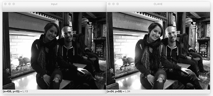
On the left, we have our original input image. We then apply adaptive histogram equalization on the right — compare these results to that of Figure 4, where we applied basic histogram equalization.
Notice how adaptive histogram equalization has improved the contrast of the input image. My wife and I are more visible. The once near-invisible couple in the background can be seen. There are fewer artifacts on my forehead, etc.
Histogram equalization suggestions
When building your own image processing pipelines and finding that histogram equalization should be applied, I suggest starting with simple histogram equalization using cv2.equalizeHist. But if you find that the results are poor and instead boost the input image’s noise, you should then try using adaptive histogram equalization through cv2.createCLAHE.
Credits
I thank Aruther Cotse (University of Utah) for the fantastic report on using histograms for image processing. Cotse’s work inspired some of the example figures in this post.
Additionally, I acknowledge the contributors to Wikipedia’s page on histogram equalization. If you’re interested in more mathematical details behind histogram equalization, be sure to refer to that page.
The example moon.png image was obtained from this article on EarthSky, while the dog.png image came from this page.
What's next? We recommend PyImageSearch University.
86+ total classes • 115+ hours hours of on-demand code walkthrough videos • Last updated: May 2026
★★★★★ 4.84 (128 Ratings) • 16,000+ Students Enrolled
I strongly believe that if you had the right teacher you could master computer vision and deep learning.
Do you think learning computer vision and deep learning has to be time-consuming, overwhelming, and complicated? Or has to involve complex mathematics and equations? Or requires a degree in computer science?
That’s not the case.
All you need to master computer vision and deep learning is for someone to explain things to you in simple, intuitive terms. And that’s exactly what I do. My mission is to change education and how complex Artificial Intelligence topics are taught.
If you're serious about learning computer vision, your next stop should be PyImageSearch University, the most comprehensive computer vision, deep learning, and OpenCV course online today. Here you’ll learn how to successfully and confidently apply computer vision to your work, research, and projects. Join me in computer vision mastery.
Inside PyImageSearch University you'll find:
- ✓ 86+ courses on essential computer vision, deep learning, and OpenCV topics
- ✓ 86 Certificates of Completion
- ✓ 115+ hours hours of on-demand video
- ✓ Brand new courses released regularly, ensuring you can keep up with state-of-the-art techniques
- ✓ Pre-configured Jupyter Notebooks in Google Colab
- ✓ Run all code examples in your web browser — works on Windows, macOS, and Linux (no dev environment configuration required!)
- ✓ Access to centralized code repos for all 540+ tutorials on PyImageSearch
- ✓ Easy one-click downloads for code, datasets, pre-trained models, etc.
- ✓ Access on mobile, laptop, desktop, etc.
Summary
In this tutorial, you learned how to perform both basic histogram equalization and adaptive histogram equalization with OpenCV.
Basic histogram equalization aims to improve the global contrast of an image by “spreading out” pixel intensities often used in the image.
But while simple histogram equalization is easy to apply and computationally efficient, the problem is that it can increase noise. What would be basic noise that could be easily filtered out is now further contaminating the signal (i.e., the components of the image we want to process).
If and when that happens, we can apply adaptive histogram equalization to obtain better results.
Adaptive histogram equalization works by dividing an image into an M x N grid and then applying histogram equalization locally to each grid. The result is an output image that overall has higher contrast with (ideally) the noise still suppressed.
To download the source code to this post (and be notified when future tutorials are published here on PyImageSearch), simply enter your email address in the form below!

Download the Source Code and FREE 17-page Resource Guide
Enter your email address below to get a .zip of the code and a FREE 17-page Resource Guide on Computer Vision, OpenCV, and Deep Learning. Inside you'll find my hand-picked tutorials, books, courses, and libraries to help you master CV and DL!


Comment section
Hey, Adrian Rosebrock here, author and creator of PyImageSearch. While I love hearing from readers, a couple years ago I made the tough decision to no longer offer 1:1 help over blog post comments.
At the time I was receiving 200+ emails per day and another 100+ blog post comments. I simply did not have the time to moderate and respond to them all, and the sheer volume of requests was taking a toll on me.
Instead, my goal is to do the most good for the computer vision, deep learning, and OpenCV community at large by focusing my time on authoring high-quality blog posts, tutorials, and books/courses.
If you need help learning computer vision and deep learning, I suggest you refer to my full catalog of books and courses — they have helped tens of thousands of developers, students, and researchers just like yourself learn Computer Vision, Deep Learning, and OpenCV.
Click here to browse my full catalog.