Ever see A Scanner Darkly?

The movie was shot digitally, but then an animated feel was given to it in the post-processing steps — but it was a painstaking process. For each frame in the movie, animators traced over the original footage, frame by frame.

Just take a second to consider the number of frames in a movie…and that each one of those frames had to be traced by hand.

Quite the undertaking, indeed.

So what if there was a way to create A Scanner Darkly animation effect using computer vision?

Is that possible?

You bet.

In this blog post I’ll show you how to use k-means clustering and color quantization to create A Scanner Darkly type effect in images.

To find out how I do it, read on.

Looking for the source code to this post?

Jump Right To The Downloads Section

OpenCV and Python versions:
This example will run on Python 2.7/Python 3.4+ and OpenCV 2.4.X/OpenCV 3.0+.

So, what is color quantization?

Color quantization is the process of reducing the number of distinct colors in an image.

Normally, the intent is to preserve the color appearance of the image as much as possible, while reducing the number of colors, whether for memory limitations or compression.

In my own work, I find that color quantization is best used when building Content-Based Image Retrieval (CBIR) systems.

If you’re unfamiliar with the term, CBIR is just a fancy academic way of saying “image search engine”.

Take a second to think about color quantization in the context of CBIR, though.

Any given 24-bit RGB image has 256 x 256 x 256 possible colors. And sure, we can build standard color histograms based on these intensity values.

But another approach is to explicitly quantize the image and reduce the number of colors to say, 16 or 64. This creates a substantially smaller space and (ideally) less noise and variance.

In practice, you can use this technique to construct more rigid color histograms.

In fact, the famous QBIC CBIR system (one of the original CBIR systems that demonstrated image search engines were possible) utilized quantized color histograms in the quadratic distance to compute similarity.

Now that we have an understanding of what color quantization is, let’s explore how we can utilize it to create A Scanner Darkly type effect in images.

Color Quantization with OpenCV

Let’s get our hands dirty.

Open up a new file, call it quant.py, and start coding:

# import the necessary packages
from sklearn.cluster import MiniBatchKMeans
import numpy as np
import argparse
import cv2

# construct the argument parser and parse the arguments
ap = argparse.ArgumentParser()
ap.add_argument("-i", "--image", required = True, help = "Path to the image")
ap.add_argument("-c", "--clusters", required = True, type = int,
	help = "# of clusters")
args = vars(ap.parse_args())

The first thing we’ll do is import our necessary packages on Lines 2-5. We’ll use NumPy for numerical processing, arparse for parsing command line arguments, and cv2 for our OpenCV bindings. Our k-means implementation will be handled by scikit-learn; specifically, the MiniBatchKMeans class.

You’ll find that MiniBatchKMeans is substantially faster than normal K-Means, although the centroids may not be as stable.

This is because MiniBatchKMeans operates on small “batches” of the dataset, whereas K-Means operates on the population of the dataset, thus making the mean calculation of each centroid, as well as the centroid update loop, much slower.

In general, I normally like to start with MiniBatchKMeans and if (and only if) my results are poor do I switch over to normal K-Means.

Lines 7-12 then handle parsing our command line arguments. We’ll need two switches: --image, which is the path to the image we want to apply color quantization to, and --clusters, which is the number of colors that our output image is going to have.

Now the real interesting code starts:

# load the image and grab its width and height
image = cv2.imread(args["image"])
(h, w) = image.shape[:2]

# convert the image from the RGB color space to the L*a*b*
# color space -- since we will be clustering using k-means
# which is based on the euclidean distance, we'll use the
# L*a*b* color space where the euclidean distance implies
# perceptual meaning
image = cv2.cvtColor(image, cv2.COLOR_BGR2LAB)

# reshape the image into a feature vector so that k-means
# can be applied
image = image.reshape((image.shape[0] * image.shape[1], 3))

# apply k-means using the specified number of clusters and
# then create the quantized image based on the predictions
clt = MiniBatchKMeans(n_clusters = args["clusters"])
labels = clt.fit_predict(image)
quant = clt.cluster_centers_.astype("uint8")[labels]

# reshape the feature vectors to images
quant = quant.reshape((h, w, 3))
image = image.reshape((h, w, 3))

# convert from L*a*b* to RGB
quant = cv2.cvtColor(quant, cv2.COLOR_LAB2BGR)
image = cv2.cvtColor(image, cv2.COLOR_LAB2BGR)

# display the images and wait for a keypress
cv2.imshow("image", np.hstack([image, quant]))
cv2.waitKey(0)

First, we load our image off disk on Line 15 and grab its height and width, respectively, on Line 16.

Line 23 handles converting our image from the RGB color space to the L*a*b* color space.

Why are we bothering doing this conversion?

Because in the L*a*b* color space the euclidean distance between colors has actual perceptual meaning — this is not the case for the RGB color space.

Given that k-means clustering also assumes a euclidean space, we’re better off using L*a*b* rather than RGB.

In order to cluster our pixel intensities, we need to reshape our image on Line 27. This line of code simply takes a (M, N, 3) image, (M x N pixels, with three components per pixel) and reshapes it into a (M x N, 3) feature vector. This reshaping is important since k-means assumes a two dimensional array, rather than a three dimensional image.

From there, we can apply our actual mini-batch K-Means clustering on Lines 31-33.

Line 31 handles instantiating our MiniBatchKMeans class using the number of clusters we specified in command line argument, whereas Line 32 performs the actual clustering.

Besides the actual clustering, Line 32 handles something extremely important — “predicting” what quantized color each pixel in the original image is going to be. This prediction is handled by determining which centroid the input pixel is closest to.

From there, we can take these predicted labels and create our quantized image on Line 33 using some fancy NumPy indexing. All this line is doing is using the predicted labels to lookup the L*a*b* color in the centroids array.

Lines 36 and 37 then handle reshaping our (M x N, 3) feature vector back into a (M, N, 3) dimensional image, followed by converting our images from the L*a*b* color space back to RGB.

Finally, Lines 44 and 45 display our original and quantized image.

Now that the coding is done, let’s take a look at the results.

Creating A Scanner Darkly Effect using Computer Vision

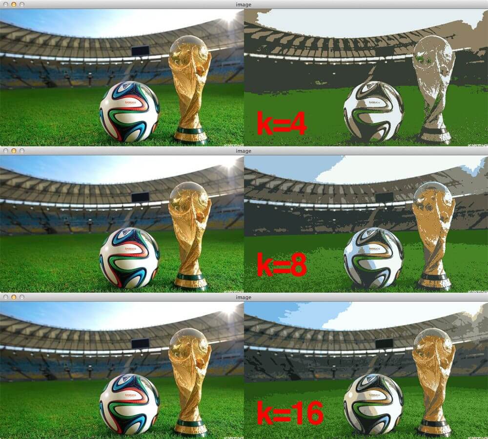
Since it’s World Cup season, let’s start with a soccer image.

Here we can see our original image on the left and our quantized image on the right.

Clearly we can see that when using only k=4 colors that we have much lost of the color detail of the original image, although an attempt is made to model the original color space of the image — the grass is still green, the soccer ball still has white in it, and the sky still has a tinge of blue.

But as we increase the k=8 and k=16 colors we can definitely start to see improved results.

It’s really interesting to note that it only takes 16 colors to create a good representation of the original image, and thus our A Scanner Darkly effect.

Let’s try another image:

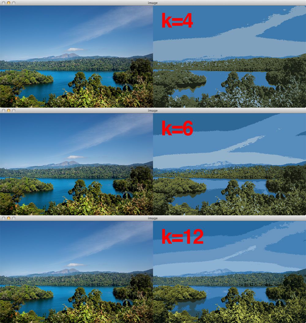
Again, the original nature scene image is on the left and the quantized output on the right.

Just like the World Cup image, notice that as the number of quantized clusters increase, we are able to better mimic the original color space.

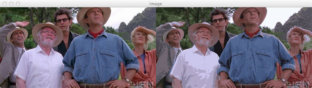
Finally, take a look at Figure 3 to see a screen capture from Jurassic Park. Notice how the number of colors have been reduced — this is explicitly evident in Hammond’s white shirt.

There is an obvious tradeoff between the number of clusters and the quality of the quantized image.

The first tradeoff is that as the number of clusters increases, so does the amount of time it takes to perform the clustering.

The second tradeoff is that as the number of clusters increases, so does the amount of memory it takes to store the output image; however, in both cases, the memory footprint will still be smaller than the original image since you are working with a substantially smaller color palette.

What's next? We recommend PyImageSearch University.

Course information:
86+ total classes • 115+ hours hours of on-demand code walkthrough videos • Last updated: March 2025
★★★★★ 4.84 (128 Ratings) • 16,000+ Students Enrolled

I strongly believe that if you had the right teacher you could master computer vision and deep learning.

Do you think learning computer vision and deep learning has to be time-consuming, overwhelming, and complicated? Or has to involve complex mathematics and equations? Or requires a degree in computer science?

That’s not the case.

All you need to master computer vision and deep learning is for someone to explain things to you in simple, intuitive terms. And that’s exactly what I do. My mission is to change education and how complex Artificial Intelligence topics are taught.

If you're serious about learning computer vision, your next stop should be PyImageSearch University, the most comprehensive computer vision, deep learning, and OpenCV course online today. Here you’ll learn how to successfully and confidently apply computer vision to your work, research, and projects. Join me in computer vision mastery.

Inside PyImageSearch University you'll find:

• ✓ 86+ courses on essential computer vision, deep learning, and OpenCV topics
• ✓ 86 Certificates of Completion
• ✓ 115+ hours hours of on-demand video
• ✓ Brand new courses released regularly, ensuring you can keep up with state-of-the-art techniques
• ✓ Pre-configured Jupyter Notebooks in Google Colab
• ✓ Run all code examples in your web browser — works on Windows, macOS, and Linux (no dev environment configuration required!)
• ✓ Access to centralized code repos for all 540+ tutorials on PyImageSearch
• ✓ Easy one-click downloads for code, datasets, pre-trained models, etc.
• ✓ Access on mobile, laptop, desktop, etc.

Click here to join PyImageSearch University

Summary

In this blog post I showed you how to perform color quantization using OpenCV and k-means clustering to create A Scanner Darkly type of effect in images.

While color quantization does not perfectly mimic the movie effect, it does demonstrate that by reducing the number of colors in an image, you can create a more posterized, animated feel to the image.

Of course, color quantization has more practical applications than just visual appeal.

Color quantization is commonly used in systems where memory is limited or when compression is required.

In my own personal work, I find that color quantization is best used when building CBIR systems. In fact, QBIC, one of the seminal image search engines, demonstrated that by using quantized color histograms and the quadratic distance, that image search engines were indeed possible.

So take a second to use the form below to download the code. And then create some quantized images of your own and send them over to me. I’m looking forward to seeing your results!

Download the Source Code and FREE 17-page Resource Guide

Enter your email address below to get a .zip of the code and a FREE 17-page Resource Guide on Computer Vision, OpenCV, and Deep Learning. Inside you'll find my hand-picked tutorials, books, courses, and libraries to help you master CV and DL!

Download the code!

Website