In this tutorial, you will learn how to perform histogram matching using OpenCV and scikit-image.

Last week we discussed histogram equalization, a basic image processing technique that can improve the contrast of an input image.
But what if you wanted to match the contrast or color distribution of two images automatically?
For example, suppose we have an input image and a reference image. Our goal is to:
- Compute histograms for each image
- Take the reference image histogram
- Update the pixel intensity values in the input image using the reference histogram, such that they match
We see the result in the figure at the top of this blog post. Notice how the input image is updated to match the color distribution of the reference image.
Histogram matching is beneficial when applying image processing pipelines to images captured in different lighting conditions, thereby creating a “normalized” representation of images, regardless of the lighting conditions they were captured in (with reasonable expectations set on how much the lighting conditions change, of course).
Today we’ll discuss histogram matching in detail. Next week I’ll show how to use histogram equalization for color correction and color constancy.
To learn how to perform histogram matching with OpenCV and scikit-image, just keep reading.
Histogram matching with OpenCV, scikit-image, and Python
In the first part of this tutorial, we’ll discuss histogram matching and implement histogram matching using OpenCV and scikit-image.
We’ll then configure our development environment and review our project directory structure.
Once we understand our project structure, we’ll implement a Python script that will:
- Load an input image (i.e., “source” image)
- Load a reference image
- Compute histograms for both images
- Take the input image and match it to the reference image, thereby transferring the color/intensity distribution from the reference image into the source image
We’ll wrap this tutorial with a discussion of our results.
What is histogram matching?

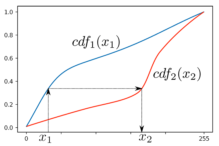
Histogram matching can best be thought of as a “transformation.” Our goal is to take an input image (the “source”) and update its pixel intensities such that the distribution of the input image histogram matches the distribution of a reference image.
While the input image’s actual contents do not change, the pixel distribution does, thereby adjusting the illumination and contrast of the input image based on the distribution of the reference image.
Applying histogram matching allows us to obtain interesting aesthetic results (as we’ll see later in this tutorial).
Additionally, we can use histogram matching as a form of basic color correction/color constancy, allowing us to build better, more reliable image processing pipelines without leveraging complex, computationally expensive machine learning and deep learning algorithms. We’ll cover that concept in next week’s guide.
How can OpenCV and scikit-image be used for histogram matching?

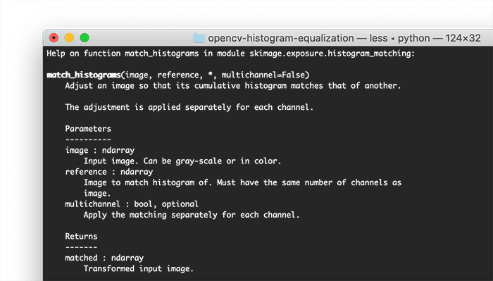
Histogram matching can be a real pain to implement by hand, but luckily for us, the scikit-image library already has a match_histograms function (the documentation you can find here).
Applying histogram matching is therefore as simple as loading two images with OpenCV’s cv2.imread and then calling scikit-image’s match_histograms function:
src = cv2.imread(args["source"])
ref = cv2.imread(args["reference"])
multi = True if src.shape[-1] > 1 else False
matched = exposure.match_histograms(src, ref, multichannel=multi)
We’ll cover how to use the match_histograms function in more detail later in this guide.
Configuring your development environment
To learn how to perform histogram matching, you need to have both OpenCV and scikit-image installed:
Both are pip-installable:
$ pip install opencv-contrib-python
$ pip install scikit-image==0.18.1
If you need help configuring your development environment for OpenCV, I highly recommend that you read my pip install OpenCV guide — it will have you up and running in a matter of minutes.
Having problems configuring your development environment?

All that said, are you:
- Short on time?
- Learning on your employer’s administratively locked system?
- Wanting to skip the hassle of fighting with the command line, package managers, and virtual environments?
- Ready to run the code right now on your Windows, macOS, or Linux systems?
Then join PyImageSearch Plus today!
Gain access to Jupyter Notebooks for this tutorial and other PyImageSearch guides that are pre-configured to run on Google Colab’s ecosystem right in your web browser! No installation required.
And best of all, these Jupyter Notebooks will run on Windows, macOS, and Linux!
Project structure
Before we can implement histogram matching with OpenCV and scikit-image, let’s first use our project directory structure.
Be sure to access the “Downloads” section of this guide to retrieve the source code and example images.
From there, take a look at our project directory structure:
$ tree . --dirsfirst
.
├── empire_state_cloudy.png
├── empire_state_sunset.png
└── match_histograms.py

0 directories, 3 files
We have only one Python script to review today, match_histograms.py, which will load empire_state_cloud.png (the source image) along with empire_state_sunset.png (the reference image).
Our script will then apply histogram matching to transfer the color distribution from the reference image onto the source image.
In this case, we’ll be able to convert a photo taken on a cloudy day to a beautiful sunset!
Implementing histogram matching with OpenCV and scikit-image
Ready to implement histogram matching?
Great, let’s get started.
Open match_histograms.py and insert the following code:
# import the necessary packages
from skimage import exposure
import matplotlib.pyplot as plt
import argparse
import cv2

# construct the argument parser and parse the arguments
ap = argparse.ArgumentParser()
ap.add_argument("-s", "--source", required=True,
	help="path to the input source image")
ap.add_argument("-r", "--reference", required=True,
	help="path to the input reference image")
args = vars(ap.parse_args())
We start on Lines 2-5, importing our required Python packages.
We need scikit-image’s exposure library to compute image histograms, cumulative distribution functions, and apply histogram matching.
We’ll use matplotlib to plot our histograms so we can visualize them before and after histogram matching is applied.
We import argparse for command line argument parsing along with cv2 for our OpenCV bindings.
Next comes our command line arguments:
--source: The path to our input image.--reference: The path to the reference image.
Keep in mind what we are doing here is taking the color distribution from the reference and then transferring it to the source. The source image is essentially the image that will have its color distribution updated.
Let’s now load our source and reference images from disk:
# load the source and reference images
print("[INFO] loading source and reference images...")
src = cv2.imread(args["source"])
ref = cv2.imread(args["reference"])

# determine if we are performing multichannel histogram matching
# and then perform histogram matching itself
print("[INFO] performing histogram matching...")
multi = True if src.shape[-1] > 1 else False
matched = exposure.match_histograms(src, ref, multichannel=multi)

# show the output images
cv2.imshow("Source", src)
cv2.imshow("Reference", ref)
cv2.imshow("Matched", matched)
cv2.waitKey(0)
Lines 17 and 18 load our src and ref images.
With these two images loaded, we can perform histogram matching on Lines 23 and 24.
Histogram matching can be applied to both single-channel and multi-channel images. Line 23 sets a Boolean, multi, depending on whether we are working with multi-channel images (True) or a single-channel image (False).
From there, applying histogram matching is as simple as calling the match_histogram function in the exposure submodule of scikit-image.
From there, Lines 27-30 display our source, reference, and output histogram matched image to our screen.
At this point, we are technically done, but to fully appreciate what histogram matching is doing, let’s examine the color histograms of the src, ref, and matched images:
# construct a figure to display the histogram plots for each channel
# before and after histogram matching was applied
(fig, axs) =  plt.subplots(nrows=3, ncols=3, figsize=(8, 8))

# loop over our source image, reference image, and output matched
# image
for (i, image) in enumerate((src, ref, matched)):
	# convert the image from BGR to RGB channel ordering
	image = cv2.cvtColor(image, cv2.COLOR_BGR2RGB)

	# loop over the names of the channels in RGB order
	for (j, color) in enumerate(("red", "green", "blue")):
		# compute a histogram for the current channel and plot it
		(hist, bins) = exposure.histogram(image[..., j],
			source_range="dtype")
		axs[j, i].plot(bins, hist / hist.max())

		# compute the cumulative distribution function for the
		# current channel and plot it
		(cdf, bins) = exposure.cumulative_distribution(image[..., j])
		axs[j, i].plot(bins, cdf)

		# set the y-axis label of the current plot to be the name
		# of the current color channel
		axs[j, 0].set_ylabel(color)
Line 34 creates a 3 x 3 figure to display the histograms of the Red, Green, and Blue channels for each of the src, ref, and matched images, respectively.
From there, Line 38 loops over each of our src, ref, and matched images. We then convert the current image from BGR to RGB channel ordering.
Next comes the actual plotting:
- Lines 45 and 46 compute a histogram for the current channel of the current
image - We then plot that histogram on Line 47
- Similarly, Lines 51 and 52 compute the cumulative distribution function of the current channel and then plot it
- Line 56 sets the y-axis label of the color
The final step is to display the plot:
# set the axes titles
axs[0, 0].set_title("Source")
axs[0, 1].set_title("Reference")
axs[0, 2].set_title("Matched")

# display the output plots
plt.tight_layout()
plt.show()
Here, we set each of the axes’ titles and then display the histogram plots on our screen.
Histogram matching results
We are now ready to apply histogram matching with OpenCV!
Be sure to access the “Downloads” section of this tutorial to retrieve the source code and example images.
From there, we open a shell and execute the following command:
$ python match_histograms.py --source empire_state_cloudy.png \
	--reference empire_state_sunset.png
[INFO] loading source and reference images...
[INFO] performing histogram matching...

Suppose we are on a family vacation to New York City, and we want to capture a beautiful photo of the Empire State Building at sunset. Today is the final day of our vacation, and our flight is scheduled to depart before lunch.
We quickly snap a photo of the Empire State Building before leaving for the airport — but it’s a cloudy, dreary day. It’s a far cry from the heavenly sunset photo we wanted.
What do we do?
The answer is to apply histogram matching.
On the flight home, we open our laptop and get to work:
- We start by loading our original input image from disk (left)
- We then hop on Google Images and find a photo of the Empire State Building at sunset (right)
- And finally, we apply histogram matching to transfer the color intensity distribution from the sunset photo (reference image) to our input image (source image)
The result is that it now looks like our original image, captured during the day time, now looks like it was captured at dusk (Figure 4)!
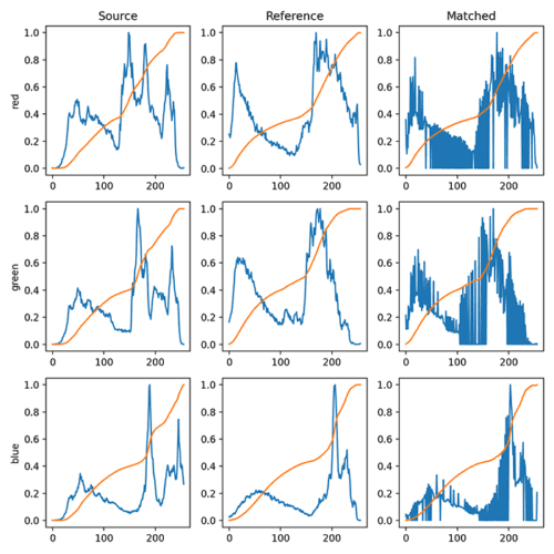
Figure 5 displays the histograms of the source, reference, and matched image for each of the Red, Green, and Blue channels of the images, respectively:

The “Source” column shows the distribution of pixel intensities in our input source image. The “Reference” column displays the distribution for the reference image we loaded from disk. And finally, the “Matched” column displays the output of applying histogram matching.
Notice how the source pixel intensities are adjusted to match the distribution of the reference image! That operation, in essence, is histogram matching.
While this tutorial focused on histogram matching from an aesthetics perspective, there are far more important real-world applications of histogram matching.
Histogram matching can be used as a normalization technique in an image processing pipeline as a form of color correction and color matching, thereby allowing you to obtain a consistent, normalized representation of images, even if lighting conditions change.
I’ll show you how to perform this type of normalization in next week’s blog post.
Credits
The source and reference images for this tutorial are credited to this article and this one. Thank you for allowing me the privilege to teach histogram matching using these example images.
Additionally, I would like to personally thank the developers and maintainers of the scikit-image library. My histogram matching implementation was based on the official example from scikit-image.
My primary contribution was to demonstrate how to use OpenCV with scikit-image’s match_histograms function and provide a more detailed discussion of the code.
What's next? We recommend PyImageSearch University.
86+ total classes • 115+ hours hours of on-demand code walkthrough videos • Last updated: May 2026
★★★★★ 4.84 (128 Ratings) • 16,000+ Students Enrolled
I strongly believe that if you had the right teacher you could master computer vision and deep learning.
Do you think learning computer vision and deep learning has to be time-consuming, overwhelming, and complicated? Or has to involve complex mathematics and equations? Or requires a degree in computer science?
That’s not the case.
All you need to master computer vision and deep learning is for someone to explain things to you in simple, intuitive terms. And that’s exactly what I do. My mission is to change education and how complex Artificial Intelligence topics are taught.
If you're serious about learning computer vision, your next stop should be PyImageSearch University, the most comprehensive computer vision, deep learning, and OpenCV course online today. Here you’ll learn how to successfully and confidently apply computer vision to your work, research, and projects. Join me in computer vision mastery.
Inside PyImageSearch University you'll find:
- ✓ 86+ courses on essential computer vision, deep learning, and OpenCV topics
- ✓ 86 Certificates of Completion
- ✓ 115+ hours hours of on-demand video
- ✓ Brand new courses released regularly, ensuring you can keep up with state-of-the-art techniques
- ✓ Pre-configured Jupyter Notebooks in Google Colab
- ✓ Run all code examples in your web browser — works on Windows, macOS, and Linux (no dev environment configuration required!)
- ✓ Access to centralized code repos for all 540+ tutorials on PyImageSearch
- ✓ Easy one-click downloads for code, datasets, pre-trained models, etc.
- ✓ Access on mobile, laptop, desktop, etc.
Summary
In this tutorial, you learned how to perform histogram matching using OpenCV and scikit-image.
Histogram matching is an image processing technique that transfers the distribution of pixel intensities from one image (the “reference” image) to another image (the “source” image).
While histogram matching can improve the aesthetics of an input image, it can also be used as a normalization technique where we “correct” an input image to make the input distribution match the reference distribution, regardless of lighting condition changes.
Performing this normalization makes our lives easier as computer vision practitioners. If we can safely assume a specific range of lighting conditions, we can hard-code parameters, including Canny edge detection thresholds, Gaussian blur sizes, etc.
I’ll show you how to perform this type of color matching and normalization in next week’s tutorial.
To download the source code to this post (and be notified when future tutorials are published here on PyImageSearch), simply enter your email address in the form below!

Download the Source Code and FREE 17-page Resource Guide
Enter your email address below to get a .zip of the code and a FREE 17-page Resource Guide on Computer Vision, OpenCV, and Deep Learning. Inside you'll find my hand-picked tutorials, books, courses, and libraries to help you master CV and DL!


Comment section
Hey, Adrian Rosebrock here, author and creator of PyImageSearch. While I love hearing from readers, a couple years ago I made the tough decision to no longer offer 1:1 help over blog post comments.
At the time I was receiving 200+ emails per day and another 100+ blog post comments. I simply did not have the time to moderate and respond to them all, and the sheer volume of requests was taking a toll on me.
Instead, my goal is to do the most good for the computer vision, deep learning, and OpenCV community at large by focusing my time on authoring high-quality blog posts, tutorials, and books/courses.
If you need help learning computer vision and deep learning, I suggest you refer to my full catalog of books and courses — they have helped tens of thousands of developers, students, and researchers just like yourself learn Computer Vision, Deep Learning, and OpenCV.
Click here to browse my full catalog.