Fine-tuning with Keras and Deep Learning

In this tutorial, you will learn how to perform fine-tuning with Keras and Deep Learning.

We will take a CNN pre-trained on the ImageNet dataset and fine-tune it to perform image classification and recognize classes it was never trained on.

Today is the final post in our three-part series on fine-tuning:

1. Part #1: Transfer learning with Keras and Deep Learning
2. Part #2: Feature extraction with on large datasets with Keras and Deep Learning
3. Part #3: Fine-tuning with Keras and Deep Learning (today’s post)

I would strongly encourage you to read the previous two tutorials in the series if you haven’t yet — understanding the concept of transfer learning, including performing feature extraction via a pre-trained CNN, will better enable you to understand (and appreciate) fine-tuning.

When performing feature extraction we did not re-train the original CNN. Instead, we treated the CNN as an arbitrary feature extractor and then trained a simple machine learning model on top of the extracted features.

Fine-tuning, on the other hand, requires that we not only update the CNN architecture but also re-train it to learn new object classes.

Fine-tuning is a multi-step process:

1. Remove the fully connected nodes at the end of the network (i.e., where the actual class label predictions are made).
2. Replace the fully connected nodes with freshly initialized ones.
3. Freeze earlier CONV layers earlier in the network (ensuring that any previous robust features learned by the CNN are not destroyed).
4. Start training, but only train the FC layer heads.
5. Optionally unfreeze some/all of the CONV layers in the network and perform a second pass of training.

If you are new to deep learning and CNNs, I would recommend you stop here and learn how to train your first CNN.

Fine-tuning with Keras is a more advanced technique with plenty of gotchas and pitfalls that will trip you up along the way (for example, it tends to be very easy to overfit a network when performing fine-tuning if you are not careful).

To learn how to perform fine-tuning with Keras and deep learning, just keep reading.

Fine-tuning with Keras and Deep Learning

2020-06-04 Update: This blog post is now TensorFlow 2+ compatible!

Note: Many of the fine-tuning concepts I’ll be covering in this post also appear in my book, Deep Learning for Computer Vision with Python. Inside the book, I go into considerably more detail (and include more of my tips, suggestions, and best practices). If you would like more detail on fine-tuning with Keras after going through this guide, definitely take a look at my book.

In the first part of this tutorial, we’ll discuss the concept of fine-tuning and how we can re-train a neural network to recognize classes it was not originally trained to recognize.

From there we’ll review the dataset we are using for fine-tuning.

I’ll then discuss our project directory structure.

Once we have a good handle on the dataset we’ll then switch to implementing fine-tuning with Keras.

After you have finished going through this tutorial you will be able to:

1. Fine-tune networks with Keras.
2. Make predictions using the fine-tuned network.

Let’s get started!

What is fine-tuning?

Note: The following section has been adapted from my book, Deep Learning for Computer Vision with Python. For the full set of chapters on transfer learning and fine-tuning, please refer to the text.

Earlier in this series of posts on transfer learning, we learned how to treat a pre-trained Convolutional Neural Network as a feature extractor.

Using this feature extractor, we forward propagated our dataset of images through the network, extracted the activations at a given layer (treating the activations as a feature vector), and then saved the values to disk.

A standard machine learning classifier (in our case, Logistic Regression), was trained on top of the CNN features, exactly as we would do with hand-engineered features such as SIFT, HOG, LBPs, etc.

This approach to transfer learning is called feature extraction.

But there is another type of transfer learning, one that can actually outperform the feature extraction method. This method is called fine-tuning and requires us to perform “network surgery”.

First, we take a scalpel and cut off the final set of fully connected layers (i.e., the “head” of the network where the class label predictions are returned) from a pre-trained CNN (typically VGG, ResNet, or Inception).

We then replace the head with a new set of fully connected layers with random initializations.

From there, all layers below the head are frozen so their weights cannot be updated (i.e., the backward pass in back propagation does not reach them).

We then train the network using a very small learning rate so the new set of fully connected layers can learn patterns from the previously learned CONV layers earlier in the network — this process is called allowing the FC layers to “warm up”.

Optionally, we may unfreeze the rest of the network and continue training. Applying fine-tuning allows us to utilize pre-trained networks to recognize classes they were not originally trained on.

And furthermore, this method can lead to higher accuracy than transfer learning via feature extraction.

Fine-tuning and network surgery

Note: The following section has been adapted from my book, Deep Learning for Computer Vision with Python. For the full set of chapters on transfer learning and fine-tuning, please refer to the text.

As we discussed earlier in this series on transfer learning via feature extraction, pre-trained networks (such as ones trained on the ImageNet dataset) contain rich, discriminative filters. The filters can be used on datasets to predict class labels outside the ones the network has already been trained on.

However, instead of simply applying feature extraction, we are going to perform network surgery and modify the actual architecture so we can re-train parts of the network.

If this sounds like something out of a bad horror movie; don’t worry, there won’t be any blood and gore — but we’ll have some fun and learn a lot about transfer learning via our Dr. Frankenstien-esque network experiments.

To understand how fine-tuning works, consider the following figure:

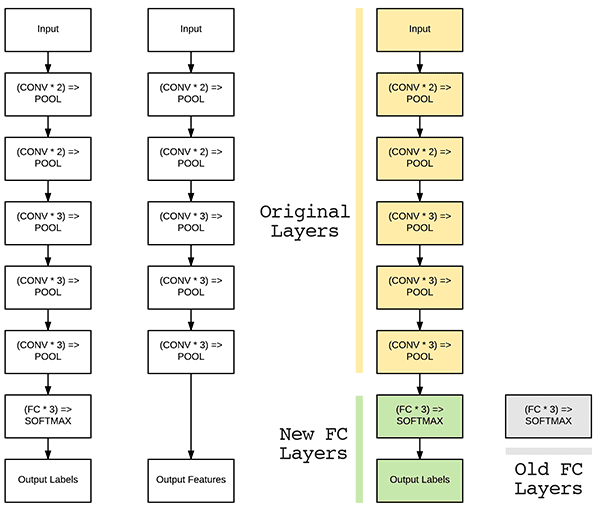
On the left we have the layers of the VGG16 network.

As we know, the final set of layers (i.e., the “head”) are our fully connected layers along with our softmax classifier.

When performing fine-tuning, we actually sever the head of the network, just as in feature extraction (Figure 2, middle).

However, unlike feature extraction, when we perform fine-tuning we actually build a new fully connected head and place it on top of the original architecture (Figure 2, right).

The new FC layer head is randomly initialized (just like any other layer in a new network) and connected to the body of the original network.

However, there is a problem:

Our CONV layers have already learned rich, discriminative filters while our FC layers are brand new and totally random.

If we allow the gradient to backpropagate from these random values all the way through the network, we risk destroying these powerful features.

To circumvent this problem, we instead let our FC head “warm up” by (ironically) “freezing” all layers in the body of the network (I told you the horror/cadaver analogy works well here) as depicted in Figure 2 (left).

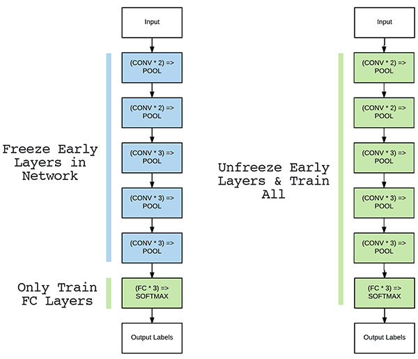
Training data is forward propagated through the network as we usually would; however, the backpropagation is stopped after the FC layers, which allows these layers to start to learn patterns from the highly discriminative CONV layers.

In some cases, we may decide to never unfreeze the body of the network as our new FC head may obtain sufficient accuracy.

However, for some datasets it is often advantageous to allow the original CONV layers to be modified during the fine-tuning process as well (Figure 3, right).

After the FC head has started to learn patterns in our dataset, we can pause training, unfreeze the body, and continue training, but with a very small learning rate — we do not want to alter our CONV filters dramatically.

Training is then allowed to continue until sufficient accuracy is obtained.

Fine-tuning is a super-powerful method to obtain image classifiers on your own custom datasets from pre-trained CNNs (and is even more powerful than transfer learning via feature extraction).

If you’d like to learn more about transfer learning via deep learning, including:

• Deep learning-based feature extraction
• Training models on top of extracted features
• Fine-tuning networks on your own custom datasets
• My personal tips, suggestions, and best practices for transfer learning

…then you’ll want to take a look at my book, Deep Learning for Computer Vision with Python, where I cover these algorithms and techniques in detail.

Configuring your development environment

To configure your system for this tutorial, I first recommend following either of these tutorials:

• How to install TensorFlow 2.0 on Ubuntu
• How to install TensorFlow 2.0 on macOS

Either tutorial will help you configure you system with all the necessary software for this blog post in a convenient Python virtual environment.

Please note that PyImageSearch does not recommend or support Windows for CV/DL projects.

2020-06-03 Update: This TensorFlow 2.0 bug affects this blog post: Filling up shuffle buffer (this may take a while). The bug has been fixed in Tensorflow 2.1 according to this GitHub issue. Please use TensorFlow >= 2.1 so that you don’t encounter this bug!

The Food-11 Dataset

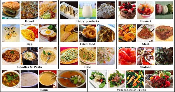
The dataset we’ll be using for fine-tuning is the Food-11 dataset from the Multimedia Signal Processing Group (MSPG) of the Swiss Federal Institute of Technology.

The dataset consists of 16,643 images belonging to 11 major food categories:

1. Bread (1724 images)
2. Dairy product (721 images)
3. Dessert (2,500 images)
4. Egg (1,648 images)
5. Fried food (1,461images)
6. Meat (2,206 images)
7. Noodles/pasta (734 images)
8. Rice (472 images)
9. Seafood (1,505 images)
10. Soup (2,500 images)
11. Vegetable/fruit (1,172 images)

Using the Food-11 dataset we can train a deep learning model capable of recognizing each major food group — such a model could be used, for example, in a mobile fitness application that automatically tracks estimated food group and caloric intake.

To train such a model, we’ll be utilizing fine-tuning with the Keras deep learning library.

Downloading the Food-11 dataset

Go ahead and grab the zip from the “Downloads” section of this blog post.

Once you’ve downloaded the source code, change directory into fine-tuning-keras :

$ unzip fine-tuning-keras.zip
$ cd fine-tuning-keras

2020-06-04 Update: In my experience, I’ve found that downloading the Food-11 dataset is unreliable from its original source. Therefore, I’m providing a direct download link to the Food-11 dataset. The option to use wget or FTP is now removed from this article.

Now, go ahead and download Food-11 using the following link:

Download Food-11

After you download the dataset, you can extract it into your project directory (fine-tuning-keras):

$ unzip Food-11.zip

Project structure

Now that we’ve downloaded the project and dataset, go ahead and navigate back to the project root. From there let’s analyze the project structure:

$ cd ..
$ tree --dirsfirst --filelimit 10
.
├── Food-11
│   ├── evaluation [3347 entries]
│   ├── training [9866 entries]
│   └── validation [3430 entries]
├── dataset
├── output
│   ├── unfrozen.png
│   └── warmup.png
├── pyimagesearch
│   ├── __init__.py
│   └── config.py
├── build_dataset.py
├── predict.py
├── Food-11.zip
└── train.py

7 directories, 8 files

Our project structure is similar to last week’s.

Our original dataset is in the Food-11/ directory. See the direct link above to download the dataset.

Executing build_dataset.py enables us to organize the Food-11 images into the dataset/ directory.

From there, we’ll use train.py to perform fine tuning.

Finally, we’ll use predict.py to make predictions on sample images using our fine-tuned network.

Each of the aforementioned scripts takes advantage of a configuration file named config.py . Let’s go ahead and learn more about the configuration script now.

Understanding our configuration file

Before we can actually fine-tune our network, we first need to create our configuration file to store important variables, including:

• Paths to the input dataset
• Class labels
• Batch size/training parameters
• Output paths, including model files, label encoders, plot histories, etc.

Since there are so many parameters that we need, I’ve opted to use a configuration file to keep our code nice and organized (versus having to utilize many command line arguments).

Our configuration file, config.py, lives in a Python module named pyimagesearch .

We keep the config.py file there for two reasons:

1. To ensure we can import the configuration into our own Python scripts
2. To keep our code tidy and organized

Note: This config file is similar to the one in last week’s and the prior week’s tutorials.

Let’s fill our config.py file now — open it up in your favorite code editor and insert the following lines:

# import the necessary packages
import os

# initialize the path to the *original* input directory of images
ORIG_INPUT_DATASET = "Food-11"

# initialize the base path to the *new* directory that will contain
# our images after computing the training and testing split
BASE_PATH = "dataset"

First, we import os , enabling us to build file/directory paths directly in this config.

The original dataset path where we extracted the Food-11 dataset is contained in ORIG_INPUT_DATASET (Line 5).

Then we specify the BASE_PATH where our organized dataset will soon reside.

From there we’ll define the names of our TRAIN , TEST , and VAL directories:

# define the names of the training, testing, and validation
# directories
TRAIN = "training"
TEST = "evaluation"
VAL = "validation"

Followed by listing the eleven CLASSES of our Food-11 dataset:

# initialize the list of class label names
CLASSES = ["Bread", "Dairy product", "Dessert", "Egg", "Fried food",
	"Meat", "Noodles/Pasta", "Rice", "Seafood", "Soup",
	"Vegetable/Fruit"]

Finally, we’ll specify our batch size and model + plot paths:

# set the batch size when fine-tuning
BATCH_SIZE = 32

# initialize the label encoder file path and the output directory to
# where the extracted features (in CSV file format) will be stored
LE_PATH = os.path.sep.join(["output", "le.cpickle"])
BASE_CSV_PATH = "output"

# set the path to the serialized model after training
MODEL_PATH = os.path.sep.join(["output", "food11.model"])

# define the path to the output training history plots
UNFROZEN_PLOT_PATH = os.path.sep.join(["output", "unfrozen.png"])
WARMUP_PLOT_PATH = os.path.sep.join(["output", "warmup.png"])

Our BATCH_SIZE of 32 represents the size of the chunks of data that will flow through our CNN.

We’ll eventually store our serialized label encoder as a pickle file (Line 27).

Our fine-tuned serialized Keras model will be exported to the MODEL_PATH (Line 31).

Similarly, we specify the paths where our warmup and unfrozen plot images will be stored (Lines 34 and 35).

Building our image dataset for fine-tuning

If we were to store the entire Food-11 dataset in memory, it would occupy ~10GB of RAM.

Most deep learning rigs should be able to handle that amount of data, but nevertheless, I’ll be showing you how to use the .flow_from_directory function with Keras to only load small batches of data from disk at a time.

However, before we can actually get to fine-tuning and re-training a network, we first must (correctly) organize our dataset of images on disk.

In order to use the .flow_from_directory function, Keras requires that we have our dataset organized using the following template:

dataset_name/class_label/example_of_class_label.jpg

And since the Food-11 dataset also provides pre-supplied data splits, our final directory structure will have the form:

dataset_name/split_name/class_label/example_of_class_label.jpg

Having the above directory structure ensures that:

1. The .flow_from_directory function will properly work.
2. Our dataset is organized into a neat, easy to follow directory structure.

In order to take the original Food-11 images and then copy them into our desired directory structure, we need the build_dataset.py script.

Let’s review that script now:

# import the necessary packages
from pyimagesearch import config
from imutils import paths
import shutil
import os

# loop over the data splits
for split in (config.TRAIN, config.TEST, config.VAL):
	# grab all image paths in the current split
	print("[INFO] processing '{} split'...".format(split))
	p = os.path.sep.join([config.ORIG_INPUT_DATASET, split])
	imagePaths = list(paths.list_images(p))

	# loop over the image paths
	for imagePath in imagePaths:
		# extract class label from the filename
		filename = imagePath.split(os.path.sep)[-1]
		label = config.CLASSES[int(filename.split("_")[0])]

		# construct the path to the output directory
		dirPath = os.path.sep.join([config.BASE_PATH, split, label])

		# if the output directory does not exist, create it
		if not os.path.exists(dirPath):
			os.makedirs(dirPath)

		# construct the path to the output image file and copy it
		p = os.path.sep.join([dirPath, filename])
		shutil.copy2(imagePath, p)

Lines 2-5 import our necessary packages, in particular, our config .

From there we loop over data splits beginning on Line 8. Inside, we:

• Extract imagePaths and each class label (Lines 11-18).
• Create a directory structure for our organized image files (Lines 21-25).
• Copy the image files into the appropriate destination (Lines 28 and 29).

This script has been reviewed in more detail inside the Transfer learning with Keras and deep learning post. If you would like more detail on the inner-workings of build_dataset.py , please refer to the previous tutorial.

---

Before continuing, make sure you have used the “Downloads” section of the tutorial to download the source code associated with this blog post.

From there, open up a terminal and execute the following command:

$ python build_dataset.py 
[INFO] processing 'training split'...
[INFO] processing 'evaluation split'...
[INFO] processing 'validation split'...

If you investigate the dataset/ directory you’ll see three directories, one for each of our respective data splits:

$ ls dataset/
evaluation		training	validation

Inside each of the data split directories you’ll also find class label subdirectories:

$ ls -l dataset/training/
Bread
Dairy product
Dessert
Egg
Fried food
Meat
Noodles
Rice
Seafood
Soup
Vegetable

And inside each of the class label subdirectories you’ll find images associated with that label:

$ ls -l dataset/training/Bread/*.jpg | head -n 5
dataset/training/Bread/0_0.jpg
dataset/training/Bread/0_1.jpg
dataset/training/Bread/0_10.jpg
dataset/training/Bread/0_100.jpg
dataset/training/Bread/0_101.jpg

Implementing fine-tuning with Keras

Now that our images are in the proper directory structure, we can perform fine-tuning with Keras.

Let’s implement the fine-tuning script inside train.py :

# set the matplotlib backend so figures can be saved in the background
import matplotlib
matplotlib.use("Agg")

# import the necessary packages
from tensorflow.keras.preprocessing.image import ImageDataGenerator
from tensorflow.keras.applications import VGG16
from tensorflow.keras.layers import Dropout
from tensorflow.keras.layers import Flatten
from tensorflow.keras.layers import Dense
from tensorflow.keras.layers import Input
from tensorflow.keras.models import Model
from tensorflow.keras.optimizers import SGD
from sklearn.metrics import classification_report
from pyimagesearch import config
from imutils import paths
import matplotlib.pyplot as plt
import numpy as np
import os

Lines 2-19 import required packages. Let’s briefly review those that are most important to the fine-tuning concepts in today’s post:

• matplotlib : We’ll be plotting our frozen and unfrozen training efforts. Line 3 sets the backend ensuring that we can save our plots to disk as image files.
• ImageDataGenerator : Allows for data augmentation. Be sure to refer to DL4CV and this blog post for more information on this class.
• VGG16 : The seminal network trained on ImageNet that we’ll be slicing and dicing with our scalpel for the purposes of fine-tuning.
• classification_report : Calculates basic statistical information upon evaluation of our model.
• config : Our custom configuration file which we reviewed in the “Understanding our configuration file” section.

Be sure to familiarize yourself with the rest of the imports as well.

With the packages at our fingertips, we’re now ready to move on. Let’s start by defining a function for plotting training history:

def plot_training(H, N, plotPath):
	# construct a plot that plots and saves the training history
	plt.style.use("ggplot")
	plt.figure()
	plt.plot(np.arange(0, N), H.history["loss"], label="train_loss")
	plt.plot(np.arange(0, N), H.history["val_loss"], label="val_loss")
	plt.plot(np.arange(0, N), H.history["accuracy"], label="train_acc")
	plt.plot(np.arange(0, N), H.history["val_accuracy"], label="val_acc")
	plt.title("Training Loss and Accuracy")
	plt.xlabel("Epoch #")
	plt.ylabel("Loss/Accuracy")
	plt.legend(loc="lower left")
	plt.savefig(plotPath)

2020-06-03 Update: In order for this plotting snippet to be TensorFlow 2+ compatible the H.history dictionary keys are updated to fully spell out “accuracy” sans “acc” (i.e., H.history["val_accuracy"] and H.history["accuracy"]). It is semi-confusing that “val” is not spelled out as “validation”; we have to learn to love and live with the API and always remember that it is a work in progress that many developers around the world contribute to.

The plot_training function is defined on Lines 21-33. This helper function will be used to construct and save a plot of our training history.

Let’s determine the total number of images in each of our splits:

# derive the paths to the training, validation, and testing
# directories
trainPath = os.path.sep.join([config.BASE_PATH, config.TRAIN])
valPath = os.path.sep.join([config.BASE_PATH, config.VAL])
testPath = os.path.sep.join([config.BASE_PATH, config.TEST])

# determine the total number of image paths in training, validation,
# and testing directories
totalTrain = len(list(paths.list_images(trainPath)))
totalVal = len(list(paths.list_images(valPath)))
totalTest = len(list(paths.list_images(testPath)))

Lines 37-39 define paths to training, validation, and testing directories, respectively.

Then, we determine the total number of images for each split via Lines 43-45 — these values will enable us to calculate the steps per epoch.

Let’s initialize our data augmentation object and establish our mean subtraction value:

# initialize the training data augmentation object
trainAug = ImageDataGenerator(
	rotation_range=30,
	zoom_range=0.15,
	width_shift_range=0.2,
	height_shift_range=0.2,
	shear_range=0.15,
	horizontal_flip=True,
	fill_mode="nearest")

# initialize the validation/testing data augmentation object (which
# we'll be adding mean subtraction to)
valAug = ImageDataGenerator()

# define the ImageNet mean subtraction (in RGB order) and set the
# the mean subtraction value for each of the data augmentation
# objects
mean = np.array([123.68, 116.779, 103.939], dtype="float32")
trainAug.mean = mean
valAug.mean = mean

The process of data augmentation is important for small datasets. In fact, it is nearly always recommended. Lines 48-55 define our training data augmentation object. The parameters specify random rotations, zooms, translations, shears, and flips to the training data as we train.

Note: A common misconception I see about data augmentation is that the random transforms of the images are then added to the original training data — that’s not the case. The random transformations performed by data augmentation are performed in-place, implying that the dataset size does not increase. These transforms are performed in-place, on the fly, during training.

Although our validation data augmentation object (Line 59) uses the same class, we do not supply any parameters (we don’t apply data augmentation to validation or testing data). The validation ImageDataGenerator will only be used for mean subtraction which is why no parameters are needed.

Next, we set the ImageNet mean subtraction values on Line 64. In this pre-processing technique, we perform a pixel-wise subtraction for all images. Mean subtraction is one of several scaling techniques I explain in the Practitioner Bundle of Deep Learning for Computer Vision with Python. In the text, we’ll even build a custom preprocessor to more efficiently accomplish mean subtraction.

Given the pixel-wise subtraction values, we prepare each of our data augmentation objects for mean subtraction (Lines 65 and 66).

Our data augmentation generators will generate data directly from their respective directories:

# initialize the training generator
trainGen = trainAug.flow_from_directory(
	trainPath,
	class_mode="categorical",
	target_size=(224, 224),
	color_mode="rgb",
	shuffle=True,
	batch_size=config.BATCH_SIZE)

# initialize the validation generator
valGen = valAug.flow_from_directory(
	valPath,
	class_mode="categorical",
	target_size=(224, 224),
	color_mode="rgb",
	shuffle=False,
	batch_size=config.BATCH_SIZE)

# initialize the testing generator
testGen = valAug.flow_from_directory(
	testPath,
	class_mode="categorical",
	target_size=(224, 224),
	color_mode="rgb",
	shuffle=False,
	batch_size=config.BATCH_SIZE)

Lines 69-93 define generators that will load batches of images from their respective, training, validation, and testing splits.

Using these generators ensures that our machine will not run out of RAM by trying to load all of the data at once.

Let’s go ahead and perform network surgery:

# load the VGG16 network, ensuring the head FC layer sets are left
# off
baseModel = VGG16(weights="imagenet", include_top=False,
	input_tensor=Input(shape=(224, 224, 3)))

# construct the head of the model that will be placed on top of the
# the base model
headModel = baseModel.output
headModel = Flatten(name="flatten")(headModel)
headModel = Dense(512, activation="relu")(headModel)
headModel = Dropout(0.5)(headModel)
headModel = Dense(len(config.CLASSES), activation="softmax")(headModel)

# place the head FC model on top of the base model (this will become
# the actual model we will train)
model = Model(inputs=baseModel.input, outputs=headModel)

First, we’ll load the VGG16 architecture (with pre-trained ImageNet weights) from disk, leaving off the fully connected layers (Lines 97 and 98). By omitting the fully connected layers, we have effectively put the network in a guillotine to behead our network as in Figure 2.

From there, we define a new fully connected layer head (Lines 102-106).

Note: If you are unfamiliar with the contents on Lines 102-106, I recommend that you read my Keras tutorial or CNN tutorial. And if you would like to immerse yourself completely into the world of deep learning, be sure to check out my highly rated deep learning book.

On Line 110 we place the new FC layer head on top of the VGG16 base network. You can think of this as adding sutures to sew the head back on to the network body after surgery.

Take the time to review the above code block carefully as it is where the heart of fine-tuning with Keras begins.

Continuing on with fine-tuning, let’s freeze all of the CONV layers in the body of VGG16:

# loop over all layers in the base model and freeze them so they will
# *not* be updated during the first training process
for layer in baseModel.layers:
	layer.trainable = False

Lines 114 and 115 freeze all CONV layers in the VGG16 base model.

Given that the base is now frozen, we’ll go ahead and train our network (only the head weights will be updated):

# compile our model (this needs to be done after our setting our
# layers to being non-trainable
print("[INFO] compiling model...")
opt = SGD(lr=1e-4, momentum=0.9)
model.compile(loss="categorical_crossentropy", optimizer=opt,
	metrics=["accuracy"])

# train the head of the network for a few epochs (all other layers
# are frozen) -- this will allow the new FC layers to start to become
# initialized with actual "learned" values versus pure random
print("[INFO] training head...")
H = model.fit(
	x=trainGen,
	steps_per_epoch=totalTrain // config.BATCH_SIZE,
	validation_data=valGen,
	validation_steps=totalVal // config.BATCH_SIZE,
	epochs=50)

# reset the testing generator and evaluate the network after
# fine-tuning just the network head
print("[INFO] evaluating after fine-tuning network head...")
testGen.reset()
predIdxs = model.predict(x=testGen,
	steps=(totalTest // config.BATCH_SIZE) + 1)
predIdxs = np.argmax(predIdxs, axis=1)
print(classification_report(testGen.classes, predIdxs,
	target_names=testGen.class_indices.keys()))
plot_training(H, 50, config.WARMUP_PLOT_PATH)

2020-06-03 Update: Per TensorFlow 2.0+, we no-longer use the .fit_generator method; it is replaced with .fit and has the same function signature (i.e., the first argument can be a Python generator object). Similarly, .predict_generator is replaced with .predict.

In this block, we train our model , keeping in mind that no weight updates will occur in the base. Only the head of the network will be tuned at this point.

In this code block, we:

• Compile the model (Lines 120-122). We use "categorical_crossentropy" for our loss function. If you are performing classification with only two classes, be sure to use "binary_crossentropy" .
• Train our network while applying data augmentation, only updating the weights for the head of the network (Lines 128-133)
• Reset our testing generator (Line 138).
• Evaluate our network on our testing data (Lines 139-141). We’ll print classification statistics in our terminal via Lines 142 and 143.
• Plot the training history via our plot_training function (Line 144).

Now let’s proceed to unfreeze the final set of CONV layers in the base model layers:

# reset our data generators
trainGen.reset()
valGen.reset()

# now that the head FC layers have been trained/initialized, lets
# unfreeze the final set of CONV layers and make them trainable
for layer in baseModel.layers[15:]:
	layer.trainable = True

# loop over the layers in the model and show which ones are trainable
# or not
for layer in baseModel.layers:
	print("{}: {}".format(layer, layer.trainable))

We start by resetting our training and validation generators (Lines 147 and 148).

We then unfreeze the final CONV layer block in VGG16 (Lines 152 and 153). Again, only the final CONV block of VGG16 is unfrozen (not the rest of the network).

Just so there is no confusion about what is going on in our network, Lines 157 and 158 will show us which layers are frozen/not frozen (i.e., trainable). The information will print out in our terminal.

Continuing on, let’s fine-tune both the final set of CONV layers and our set of FC layers:

# for the changes to the model to take affect we need to recompile
# the model, this time using SGD with a *very* small learning rate
print("[INFO] re-compiling model...")
opt = SGD(lr=1e-4, momentum=0.9)
model.compile(loss="categorical_crossentropy", optimizer=opt,
	metrics=["accuracy"])

# train the model again, this time fine-tuning *both* the final set
# of CONV layers along with our set of FC layers
H = model.fit(
	x=trainGen,
	steps_per_epoch=totalTrain // config.BATCH_SIZE,
	validation_data=valGen,
	validation_steps=totalVal // config.BATCH_SIZE,
	epochs=20)

2020-06-03 Update: Per TensorFlow 2.0+, we no-longer use the .fit_generator method; it is replaced with .fit and has the same function signature (i.e., the first argument can be a Python generator object).

Since we’ve unfrozen additional layers, we must re-compile the model (Lines 163-165).

We then train the model again, this time fine-tuning both the FC layer head and the final CONV block (Lines 169-174).

Wrapping up, let’s evaluate the network once more:

# reset the testing generator and then use our trained model to
# make predictions on the data
print("[INFO] evaluating after fine-tuning network...")
testGen.reset()
predIdxs = model.predict(x=testGen,
	steps=(totalTest // config.BATCH_SIZE) + 1)
predIdxs = np.argmax(predIdxs, axis=1)
print(classification_report(testGen.classes, predIdxs,
	target_names=testGen.class_indices.keys()))
plot_training(H, 20, config.UNFROZEN_PLOT_PATH)

# serialize the model to disk
print("[INFO] serializing network...")
model.save(config.MODEL_PATH, save_format="h5")

2020-06-03 Update: Per TensorFlow 2.0+, we no-longer use the .predict_generator; it is replaced with .predict. and has the same function signature (i.e., the first argument can be a Python generator object).

Here we:

• Make predictions on the testing data (Lines 179-182).
• Print a new classification report (Lines 183 and 184).
• Generate the unfrozen training and save it to disk (Line 185).
• And serialize the model to disk, allowing us to recall the model in our predict.py script (Line 189).

Great job sticking with me on our fine-tuning journey. We’re going to put our script to work next!

Training a network via fine-tuning with Keras

Now that we’ve implemented our Python script to perform fine-tuning, let’s give it a try and see what happens.

Make sure you’ve used the “Downloads” section of this tutorial to download the source code to this post, and from there, execute the following command:

$ python train.py
Using TensorFlow backend.
Found 9866 images belonging to 11 classes.
Found 3430 images belonging to 11 classes.
Found 3347 images belonging to 11 classes.
[INFO] compiling model...
[INFO] training head...
Epoch 1/50
308/308 [==============================] - 91s 294ms/step - loss: 4.5022 - accuracy: 0.2844 - val_loss: 1.7583 - val_accuracy: 0.4238
Epoch 2/50
308/308 [==============================] - 89s 289ms/step - loss: 1.9905 - accuracy: 0.3551 - val_loss: 1.4969 - val_accuracy: 0.4909
Epoch 3/50 
308/308 [==============================] - 90s 294ms/step - loss: 1.8038 - accuracy: 0.3991 - val_loss: 1.4215 - val_accuracy: 0.5301
...
Epoch 48/50
308/308 [==============================] - 88s 285ms/step - loss: 0.9199 - accuracy: 0.6909 - val_loss: 0.7735 - val_accuracy: 0.7614
Epoch 49/50
308/308 [==============================] - 87s 284ms/step - loss: 0.8974 - accuracy: 0.6977 - val_loss: 0.7749 - val_accuracy: 0.7602
Epoch 50/50
308/308 [==============================] - 88s 287ms/step - loss: 0.8930 - accuracy: 0.7004 - val_loss: 0.7764 - val_accuracy: 0.7646
[INFO] evaluating after fine-tuning network head...
               precision    recall  f1-score   support

        Bread       0.72      0.58      0.64       368
Dairy product       0.75      0.56      0.64       148
      Dessert       0.72      0.68      0.70       500
          Egg       0.66      0.72      0.69       335
   Fried food       0.72      0.70      0.71       287
         Meat       0.75      0.84      0.79       432
      Noodles       0.97      0.95      0.96       147
         Rice       0.85      0.88      0.86        96
      Seafood       0.79      0.81      0.80       303
         Soup       0.89      0.95      0.92       500
    Vegetable       0.86      0.91      0.88       231

     accuracy                           0.78      3347
    macro avg       0.79      0.78      0.78      3347
 weighted avg       0.78      0.78      0.77      3347

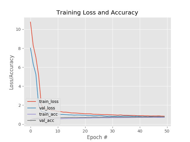
After fine-tuning just our newly initialized FC layer head and allowing the FC Layers to warm up, we are obtaining ~76% accuracy which is quite respectable.

Next, we see that we have unfrozen the final block of CONV layers in VGG16 while leaving the rest of the network weights frozen:

<tensorflow.python.keras.engine.input_layer.InputLayer object at 0x7f2baa5f6eb8>: False
<tensorflow.python.keras.layers.convolutional.Conv2D object at 0x7f2c21583198>: False
<tensorflow.python.keras.layers.convolutional.Conv2D object at 0x7f2c8075ffd0>: False
<tensorflow.python.keras.layers.pooling.MaxPooling2D object at 0x7f2c80725630>: False
<tensorflow.python.keras.layers.convolutional.Conv2D object at 0x7f2c807254a8>: False
<tensorflow.python.keras.layers.convolutional.Conv2D object at 0x7f2c8072f828>: False
<tensorflow.python.keras.layers.pooling.MaxPooling2D object at 0x7f2c807399b0>: False
<tensorflow.python.keras.layers.convolutional.Conv2D object at 0x7f2c80739828>: False
<tensorflow.python.keras.layers.convolutional.Conv2D object at 0x7f2c804c0b70>: False
<tensorflow.python.keras.layers.convolutional.Conv2D object at 0x7f2c804c52b0>: False
<tensorflow.python.keras.layers.pooling.MaxPooling2D object at 0x7f2c804cd0f0>: False
<tensorflow.python.keras.layers.convolutional.Conv2D object at 0x7f2c804cdac8>: False
<tensorflow.python.keras.layers.convolutional.Conv2D object at 0x7f2c804d4dd8>: False
<tensorflow.python.keras.layers.convolutional.Conv2D object at 0x7f2c804d94a8>: False
<tensorflow.python.keras.layers.pooling.MaxPooling2D object at 0x7f2c804de3c8>: False
<tensorflow.python.keras.layers.convolutional.Conv2D object at 0x7f2c804e2cf8>: True
<tensorflow.python.keras.layers.convolutional.Conv2D object at 0x7f2c804e2e10>: True
<tensorflow.python.keras.layers.convolutional.Conv2D object at 0x7f2c804ed828>: True
<tensorflow.python.keras.layers.pooling.MaxPooling2D object at 0x7f2c804f2550>: True

Once we’ve unfrozen the final CONV block, we resume fine-tuning:

[INFO] re-compiling model...
Epoch 1/20
308/308 [==============================] - 88s 285ms/step - loss: 0.9120 - accuracy: 0.6978 - val_loss: 0.7333 - val_accuracy: 0.7818
Epoch 2/20
308/308 [==============================] - 88s 285ms/step - loss: 0.8302 - accuracy: 0.7252 - val_loss: 0.6916 - val_accuracy: 0.7941
Epoch 3/20
308/308 [==============================] - 88s 285ms/step - loss: 0.7882 - accuracy: 0.7401 - val_loss: 0.6982 - val_accuracy: 0.7953
Epoch 4/20
308/308 [==============================] - 88s 285ms/step - loss: 0.7418 - accuracy: 0.7557 - val_loss: 0.6813 - val_accuracy: 0.8110
Epoch 5/20
308/308 [==============================] - 88s 285ms/step - loss: 0.6744 - accuracy: 0.7808 - val_loss: 0.6259 - val_accuracy: 0.8195
...
Epoch 16/20
308/308 [==============================] - 89s 289ms/step - loss: 0.4534 - accuracy: 0.8537 - val_loss: 0.5958 - val_accuracy: 0.8516
Epoch 17/20
308/308 [==============================] - 88s 285ms/step - loss: 0.4332 - accuracy: 0.8608 - val_loss: 0.5809 - val_accuracy: 0.8537
Epoch 18/20
308/308 [==============================] - 88s 285ms/step - loss: 0.4188 - accuracy: 0.8646 - val_loss: 0.6200 - val_accuracy: 0.8490
Epoch 19/20
308/308 [==============================] - 88s 285ms/step - loss: 0.4115 - accuracy: 0.8641 - val_loss: 0.5874 - val_accuracy: 0.8493
Epoch 20/20
308/308 [==============================] - 88s 285ms/step - loss: 0.3807 - accuracy: 0.8721 - val_loss: 0.5939 - val_accuracy: 0.8581
[INFO] evaluating after fine-tuning network...
               precision    recall  f1-score   support

        Bread       0.84      0.79      0.81       368
Dairy product       0.85      0.70      0.77       148
      Dessert       0.82      0.82      0.82       500
          Egg       0.84      0.84      0.84       335
   Fried food       0.82      0.86      0.84       287
         Meat       0.87      0.92      0.89       432
      Noodles       1.00      0.97      0.98       147
         Rice       0.91      0.97      0.94        96
      Seafood       0.91      0.90      0.91       303
         Soup       0.96      0.96      0.96       500
    Vegetable       0.92      0.95      0.94       231

     accuracy                           0.88      3347
    macro avg       0.89      0.88      0.88      3347
 weighted avg       0.88      0.88      0.88      3347

[INFO] serializing network...

I decided to not train past epoch 20 for fear of overfitting. If you take a look at Figure 7 you can start to see our training and validation loss start to rapidly divide. When you see training loss falling quickly while validation loss stagnates or even increases, you know you are overfitting.

That said, at the end of our fine-tuning process, we are now obtaining 88% accuracy, a significant increase from just fine-tuning the FC layer heads alone!

Making predictions with fine-tuning and Keras

Now that we’ve fine-tuned our Keras model, let’s see how we can use it to make predictions on images outside the training/testing set (i.e., our own custom images).

Open up predict.py and insert the following code:

# import the necessary packages
from tensorflow.keras.models import load_model
from pyimagesearch import config
import numpy as np
import argparse
import imutils
import cv2

# construct the argument parser and parse the arguments
ap = argparse.ArgumentParser()
ap.add_argument("-i", "--image", type=str, required=True,
	help="path to our input image")
args = vars(ap.parse_args())

Lines 2-7 import our required packages. We’re going to use load_model to recall our Keras fine-tuned model from disk and make predictions. This is also the first time today that we will use OpenCV (cv2 ).

On Lines 10-13 we parse our command line argument. The --image argument allows us to supply any image from our terminal at runtime with no modifications to the code. It makes sense to take advantage of a command line argument rather than hard-coding the value here or in our config.

Let’s go ahead and load that image from disk and preprocess it:

# load the input image and then clone it so we can draw on it later
image = cv2.imread(args["image"])
output = image.copy()
output = imutils.resize(output, width=400)

# our model was trained on RGB ordered images but OpenCV represents
# images in BGR order, so swap the channels, and then resize to
# 224x224 (the input dimensions for VGG16)
image = cv2.cvtColor(image, cv2.COLOR_BGR2RGB)
image = cv2.resize(image, (224, 224))

# convert the image to a floating point data type and perform mean
# subtraction
image = image.astype("float32")
mean = np.array([123.68, 116.779, 103.939][::-1], dtype="float32")
image -= mean

Lines 16-30 load and preprocess our image . The preprocessing steps are identical to training and include:

• Making a copy of the image and resizing it for output purposes (Lines 17 and 18).
• Swapping color channels since we trained with RGB images and OpenCV loaded this image in BGR order (Line 23).
• Resizing the image to 224×224 pixels for inference (Line 24).
• Converting the image to floating point (Line 28).
• Performing mean subtraction (Lines 29 and 30).

Note: When we perform inference using a custom prediction script, if the results are unsatisfactory nine times out of ten it is due to improper preprocessing. Typically having color channels in the wrong order or forgetting to perform mean subtraction altogether will lead to unfavorable results. Keep this in mind when writing your own scripts.

Now that our image is ready, let’s predict its class label:

# load the trained model from disk
print("[INFO] loading model...")
model = load_model(config.MODEL_PATH)

# pass the image through the network to obtain our predictions
preds = model.predict(np.expand_dims(image, axis=0))[0]
i = np.argmax(preds)
label = config.CLASSES[i]

# draw the prediction on the output image
text = "{}: {:.2f}%".format(label, preds[i] * 100)
cv2.putText(output, text, (3, 20), cv2.FONT_HERSHEY_SIMPLEX, 0.5,
	(0, 255, 0), 2)

# show the output image
cv2.imshow("Output", output)
cv2.waitKey(0)

We load our fine-tuned model via Line 34 and then perform inference. The top prediction class label is extracted on Lines 37-39.

Finally, we annotate the output image and display it on screen (Lines 42-48). The text annotation contains the highest prediction along with its associated confidence.

On to the fun part — testing our script on food! I’m hungry just thinking about it and I bet you may be too.

Keras fine-tuning results

To see our fine-tuned Keras model in action, make sure you use the “Downloads” section of this tutorial to download the source code and example images.

From there, open up a terminal and execute the following command:

$ python predict.py --image dataset/evaluation/Seafood/8_186.jpg

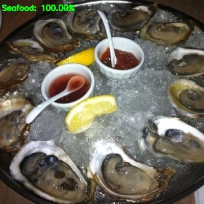
As you can see from Figure 7, we have correctly classified the input image as “Seafood”.

Let’s try another example:

$ python predict.py --image dataset/evaluation/Meat/5_293.jpg

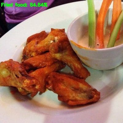
Our fine-tuned network has labeled the image as “Fried food” despite it being in the “Meat” class in our dataset.

Chicken wings are typically fried and these ones clearly are. They are both “Meat” and “Fried food” which is why we are pulled in two directions. Therefore, I’m still declaring it as a “correct” classification. A fun experiment would be to apply fine-tuning with multi-label classification. I’ll leave that as an exercise to you to implement.

Below I have included a few additional results from my fine-tuning experiments:

Summary

In this tutorial, you learned how to perform fine-tuning with Keras and deep learning.

To perform fine-tuning, we:

1. Loaded the VGG16 network architecture from disk with weights pre-trained on ImageNet.
2. Ensured the original fully connected layer heads were removed (i.e., where the output predictions from the network are made).
3. Replaced the originally fully connected layers with brand new, freshly initialized ones.
4. Froze all CONV layers in VGG16.
5. Trained only the fully connected layer heads.
6. Unfroze the final set of CONV layer blocks in VGG16.
7. Continued training.

Overall, we were able to obtain 88% accuracy on the Food-11 dataset.

Further accuracy can be obtained by applying additional data augmentation and adjusting the parameters to our optimizer and number of FC layer nodes.

If you’re interested in learning more about fine-tuning with Keras, including my tips, suggestions, and best practices, be sure to take a look at Deep Learning for Computer Vision with Python where I cover fine-tuning in more detail.

I hope you enjoyed today’s tutorial on fine-tuning!

To download the source code to this post (and be notified when future tutorials are published here on PyImageSearch), just enter your email address in the form below!