Google DeepMind’s Gemma 4: MoE, Efficiency Tricks, and Benchmarks

---

---

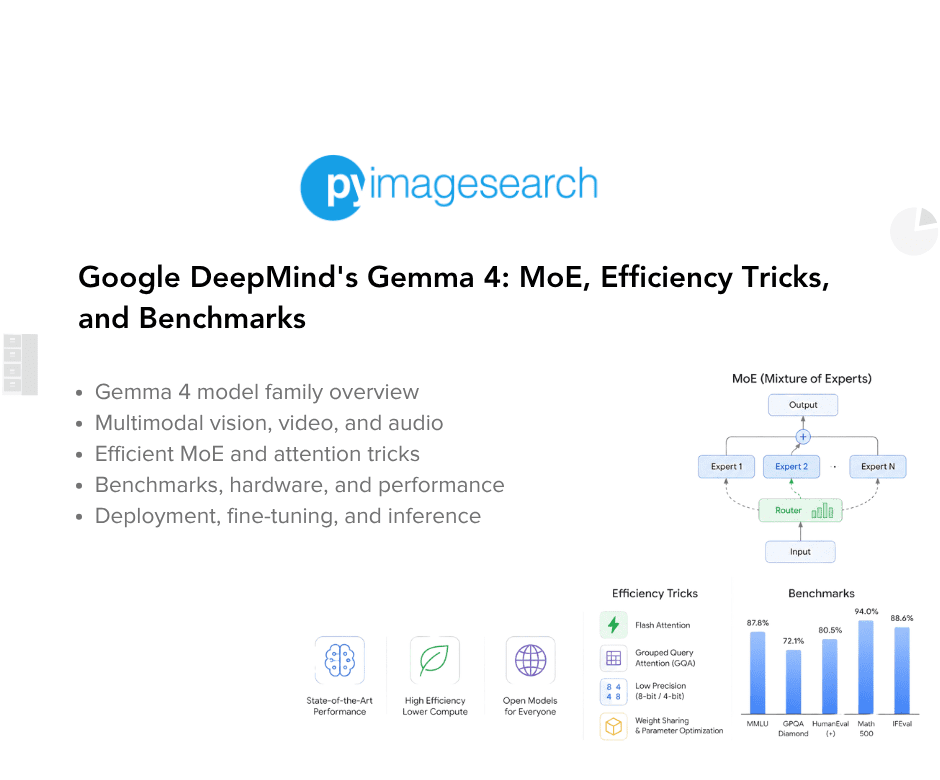
Google DeepMind’s Gemma 4: MoE, Efficiency Tricks, and Benchmarks

Google DeepMind’s Gemma 4 is one of the most compelling open-weight model releases in recent memory. It’s not just one model; it is a carefully designed family spanning from tiny on-device variants to a 31-billion-parameter powerhouse, all built with multimodal reasoning, long context, and real deployment constraints in mind. And crucially, these models are released under an Apache 2.0 license, meaning you can use, modify, and deploy them commercially without restriction.

In this post, we will peel back the hood and explain what makes Gemma 4 tick, including the architecture, the clever efficiency tricks, the multimodal capabilities, what hardware you actually need to run these models, and how to get started in code. No prior deep knowledge of transformers required, though some familiarity will help.

Whether you are evaluating Gemma 4 for a production use case, curious about the architecture, or just want to know which variant to reach for, this post has you covered.

This lesson is the 1st in a 5-part series on Google DeepMind’s Gemma 4:

1. Google DeepMind’s Gemma 4: MoE, Efficiency Tricks, and Benchmarks (this tutorial)
2. Lesson 2
3. Lesson 3
4. Lesson 4
5. Lesson 5

To learn how Gemma 4’s architecture, Mixture-of-Experts design, multimodal capabilities, and efficiency optimizations work, just keep reading.

---

Would you like immediate access to 3,457 images curated and labeled with hand gestures to train, explore, and experiment with … for free? Head over to Roboflow and get a free account to grab these hand gesture images.

---

Need Help Configuring Your Development Environment?

All that said, are you:

• Short on time?
• Learning on your employer’s administratively locked system?
• Wanting to skip the hassle of fighting with the command line, package managers, and virtual environments?
• Ready to run the code immediately on your Windows, macOS, or Linux system?

Then join PyImageSearch University today!

Gain access to Jupyter Notebooks for this tutorial and other PyImageSearch guides pre-configured to run on Google Colab’s ecosystem right in your web browser! No installation required.

And best of all, these Jupyter Notebooks will run on Windows, macOS, and Linux!

---

Gemma 4 Model Family Overview: E2B, E4B, 31B, and MoE 26B A4B

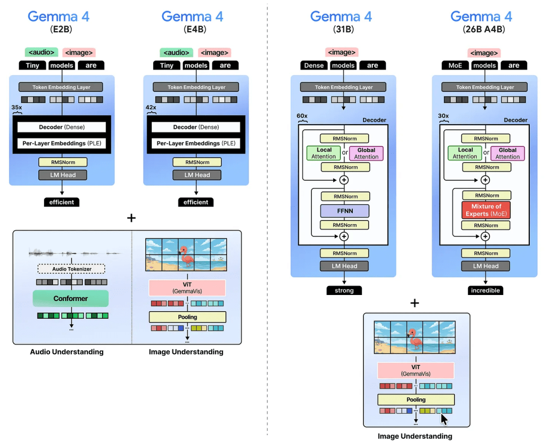
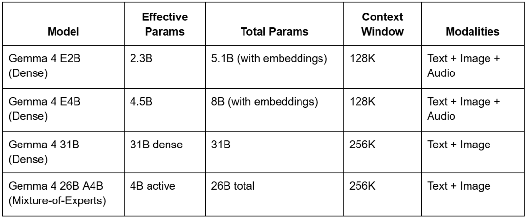
Before diving into how these models work, let us first look at the lineup. There are 4 models:

Gemma 4 E2B and E4B: The smallest models in the family, designed to run efficiently on-device (think: your phone). The “E” stands for effective parameters, a concept we’ll unpack below. They support text, images, and even audio.

Gemma 4 31B: A dense 31-billion parameter model. Dense means every parameter participates in every inference pass. Think of it as the “traditional” heavyweight.

Gemma 4 26B A4B: A Mixture-of-Experts model with 26 billion total parameters, but only 4 billion “active” during any given computation (inference). The “A” stands for active parameters. It runs with the speed of a 4B model despite its much larger knowledge capacity.

The lineup spans from phone-friendly to server-grade, so you can pick the right model for your constraints. All 4 models are multimodal; they can reason over images alongside text. The 2 smaller models (E2B and E4B) go a step further and also handle audio.

Every model ships in both a base (pre-trained) and instruction-tuned (IT) version. The instruction-tuned versions are what most practitioners will want to use for tasks like chat, reasoning, and function-calling.

All 4 models are available on Hugging Face, Kaggle, Ollama, LM Studio, and Docker. Also, it can run via Transformers, llama.cpp, MLX, and several other popular inference stacks.

---

Gemma 4 Capabilities: Reasoning, Multimodal AI, and Thinking Mode

Before getting into architecture, it is worth understanding the capabilities these models were trained and evaluated for. The design choices only make sense in that context.

---

Gemma 4 Thinking Mode: Chain-of-Thought Reasoning Explained

All Gemma 4 models are designed as capable reasoners with configurable “thinking mode.” When enabled, the model produces an internal chain-of-thought before arriving at its final answer, similar in spirit to what you would see with OpenAI’s o-series or Anthropic’s extended thinking. This is particularly valuable for math, logic, and multi-step planning tasks.

Thinking can be toggled per-request. In the Transformers API, you enable it by passing enable_thinking=True to the apply_chat_template call:

inputs = processor.apply_chat_template(
    messages,
    tokenize=True,
    return_dict=True,
    return_tensors="pt",
    add_generation_prompt=True,
    enable_thinking=True,  # activates chain-of-thought mode
).to(model.device)

---

Image Understanding: Object Detection, OCR, and GUI Navigation

The vision capabilities in Gemma 4 are genuinely impressive, especially for an open-weight model. All 4 model sizes could reliably perform bounding-box detection, returning results natively as structured JSON without any special grammar constraints or prompting tricks.

For example, given a UI screenshot and the prompt “What’s the bounding box for the ‘submit’ button?”, the model returns something like:

[{"box_2d": [171, 75, 245, 308], "label": "view recipe element"}]

The coordinates are normalized to a 1000×1000 grid regardless of the original image dimensions, which makes post-processing straightforward. This makes Gemma 4 a strong candidate for tasks like automated UI testing, document parsing, and robotic process automation.

Image captioning was tested across all 4 sizes and all performed well, accurately capturing details such as the type of bird, the architectural style of background buildings, and whether the scene was indoors or outdoors. Even the tiny E2B model produced detailed and accurate captions.

---

Gemma 4 Code Generation from Images: UI Reconstruction and Vision-to-Code

One standout test: When given each model a screenshot of a webpage and asked it to write the HTML to recreate it. With thinking mode enabled and a token budget of 4,000 output tokens, the larger models (26B A4B and 31B) produced near-faithful reproductions. The smaller E4B model held its own remarkably well, while E2B showed the expected drop-off in fidelity.

This capability to understand a visual layout and translate it into working code has real applications for prototyping, design-to-code workflows, and accessibility tooling.

---

Gemma 4 Video Understanding: Multimodal Temporal Reasoning

Gemma 4 can process video input, though capabilities differ by size. The smaller E2B and E4B models accept video with audio, treating it as a combined audio-visual signal. The larger 31B and 26B A4B models accept video without audio because they lack an audio encoder, which we will discuss below.

In informal testing with a live concert video, E4B correctly identified the genre of music, the mood of the song lyrics, and the stage setup and crowd. The 31B model gave a detailed description of the visual elements and even identified a brand visible on a large screen, despite not having access to audio. Neither model had been explicitly fine-tuned on video data; this capability emerged from the multimodal training.

---

Gemma 4 Audio AI: Speech Recognition, Translation, and Audio Q&A

The E2B and E4B models include a dedicated audio encoder, enabling end-to-end speech understanding. This is novel for an open-weight model at this scale. Practically, it means you can send raw audio (as an MP4 or audio file) and ask the model questions about the audio, with no separate transcription step required.

This is particularly useful for:

• Automatic speech recognition (ASR) in a single-model pipeline
• Multilingual audio translation
• Video Q&A where both the speech and visuals matter

---

Gemma 4 Function Calling: Tool Use and Agentic AI Workflows

Gemma 4 has built-in support for structured function/tool calling, both in text-only and multimodal contexts. This is essential for building agents: systems in which the model needs to decide which tool to invoke, with what arguments, in response to a user request. The fact that this is natively supported (rather than requiring prompt-engineering workarounds) makes Gemma 4 a serious option for agentic workflows running locally or in constrained environments.

---

Gemma 4 System Prompts: Instruction Control and Chat Behavior

Gemma 4 introduces first-class support for the system role in conversations. In prior Gemma versions, system-level instructions had to be blended into the user turn in ad hoc ways. Now the model is trained to recognize and respect a proper system prompt, which makes deploying it inside structured applications (where you want to set tone, persona, or capabilities) significantly cleaner.

---

Gemma 4 Architecture Overview: Shared Transformer Design Principles

Despite their size differences, all Gemma 4 models share the same core architectural DNA. Let us go through each shared component one by one.

---

Gemma 4 Attention Mechanism: Local + Global Interleaved Attention Explained

To appreciate what Gemma 4 does here, you first need to understand what “attention” means in a transformer model.

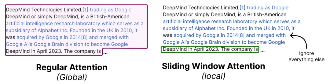
The classic attention problem: In a standard transformer, every word in your input looks at every other word to figure out context. This is called full or global attention. It is powerful but brutally expensive because the computation grows with the square of the input length. Double your input length, and you quadruple the cost.

Sliding window attention (local attention): Imagine reading a book, but instead of remembering every page you’ve ever read, you can only reference the last 5 pages. That’s sliding window attention. Each token only attends to the N most recent tokens (a “window”), not the entire sequence. This is dramatically cheaper to compute.

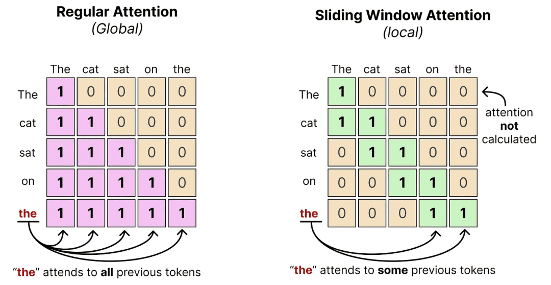
Here is the tradeoff made tangible: say you are generating a response to a long legal document. With a sliding window of 512 tokens, any given token looks only at the 512 tokens before it, rather than the entire 10,000-token document. That saves enormous compute, but risks losing context from early in the document.

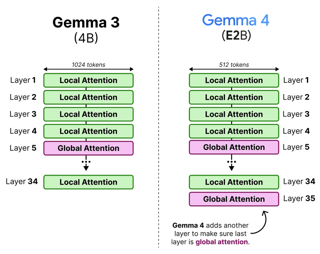
The interleaving solution: Gemma 4 does not pick one strategy; it alternates between them across layers. Most layers use the efficient sliding window, but every few layers, a full global attention layer kicks in and “resets” the context by attending to everything. Think of it like a student who mostly skims through dense reading, but every few chapters pauses to re-read everything they have covered.

In practice, the E2B model uses a 4-local-to-1-global pattern. All other models use a 5:1 ratio. Crucially, Gemma 4 ensures the final layer is always a global attention layer, so the model’s last word on any sequence is fully informed, a deliberate fix from Gemma 3 where the last layer could end up being local.

---

Gemma 4 Efficiency Tricks: GQA, K=V Caching, and Memory Optimization

Even with interleaving, global attention layers are still the most expensive part. Gemma 4 layers on three additional tricks to tame the cost.

Grouped Query Attention (GQA)

In standard multi-head attention, every “head” maintains its own set of Key and Value matrices. This creates a large memory footprint because all of these have to be cached during generation (this is called the KV-cache).

GQA is the idea that multiple Query heads can share the same set of Keys and Values. Imagine 8 students all reading from the same textbook instead of each having their own, with the same knowledge and much less paper.

In Gemma 4’s global attention layers, 8 Query heads share a single KV pair. This dramatically reduces what needs to be stored in the cache, which is especially significant because global attention has to cache the entire context (versus the local attention layers, which only cache a small window).

To compensate for any quality loss from fewer KV heads, Gemma 4 doubles the dimensionality of the Keys, giving each shared Key more expressive capacity.

Keys Equal Values (K=V)

Here’s an even bolder efficiency move: in global attention layers, Gemma 4 sets the Key and Value matrices to be identical. Instead of storing both K and V separately in cache, you only need to store one. The KV-cache effectively becomes a K-cache for those layers, cutting memory requirements in half at that level.

This sounds like it might hurt quality significantly, but in practice the performance impact turns out to be modest, a good trade for the memory savings.

p-RoPE: Smarter Positional Encoding

To understand this trick, you need to know how transformers track word order. Because attention has no built-in sense of sequence (unlike an RNN), position is injected into embeddings explicitly. The popular method for this is Rotary Positional Encoding (RoPE).

How RoPE works: Each embedding vector is split into pairs of values. Each pair is thought of as a 2D vector pointing in some direction. RoPE rotates each pair by a position-dependent angle, so earlier words get one rotation, later words get another. By comparing how much two vectors have been rotated, the model can infer their relative distance.

The rotation speeds vary: the first pairs rotate quickly (high frequency) and the last pairs rotate very slowly (low frequency). The high-frequency pairs are great for tracking where a word is. The low-frequency pairs rotate so little that they barely carry positional information at all, making them closer to the raw semantic meaning of the word.

Here is the problem Gemma 4 solves: over very long sequences, even those tiny low-frequency rotations accumulate and start to introduce misleading positional noise into what should be a semantic signal. Think of it like a clock’s hour hand being used to measure seconds, where the movement is technically there but too small to be meaningful and can cause errors.

p-RoPE (pruned RoPE) solves this elegantly: apply rotational encoding only to the first p fraction of pairs, and zero out the rest. If p = 0.25, only the top 25% of pairs (the high-frequency, positional ones) get rotation. The low-frequency pairs are left clean, with pure semantic content and no positional noise. This is especially important in global attention, where the context can span tens of thousands of tokens.

---

Gemma 4 Vision Encoder: ViT-Based Image Processing Architecture

All four Gemma 4 models are multimodal, meaning they can reason about images as well as text. To make this work, images need to be converted into a format the language model can process. The component responsible for this is the Vision Encoder, built on a Vision Transformer (ViT).

The core idea of a ViT: Rather than treating an image as a grid of pixels, a ViT slices the image into fixed-size patches (typically 16×16 pixels each) and treats each patch like a “word token.” The sequence of patches goes through a transformer, which produces an embedding for each patch capturing its visual content and context.

Handling Variable Aspect Ratios with 2D RoPE

Standard ViTs assume a square input image with a fixed grid of patches. But real-world images come in all shapes (e.g., wide panoramas, tall portraits, and square thumbnails). Forcing every image into a square distorts content and destroys spatial relationships.

Gemma 4 addresses this by using 2D RoPE for its vision encoder. Instead of encoding patches with a single 1D position (patch 1, patch 2, patch 3, etc.), each patch is given a 2D position: its (row, column) coordinates in the image grid. The patch embedding is split into two halves where one half encodes the horizontal position, and the other encodes the vertical position. This way, a patch in the upper-left corner of a wide landscape and a patch in the upper-left corner of a tall portrait both correctly identify themselves as “top-left,” regardless of the total number of patches.

Images are also adaptively resized to maintain the original aspect ratio while ensuring the dimensions are multiples of 16 (the patch size), with padding added where needed.

Soft Token Budget: Controlling Variable Resolution

More patches mean more tokens fed into the language model, which increases computational cost. To give developers control over this, Gemma 4 introduces a soft token budget: a configurable cap on how many visual tokens are processed by the LLM.

Here’s a concrete example. Suppose you set a budget of 280 tokens. The model will resize your image so that the total resulting patches, after pooling every 3×3 patch block into a single embedding, stays within 280. A budget of 1120 tokens lets high-resolution images through with much more visual detail; a budget of 70 tokens dramatically downsamples the image. The right budget depends on your task:

• Describing a photo? 70–140 tokens is probably fine.
• Reading a scanned invoice with fine print? You’d want 560–1120 tokens.
• Analyzing consecutive video frames quickly? Lower budgets keep things fast.

Linear Projection: Bridging Vision and Language

The patch embeddings produced by the ViT live in a different dimensional space than the word embeddings Gemma 4 was trained on. Feeding mismatched embeddings into the language model would be like asking someone to add meters and kilograms, which makes no sense.

To solve this, a small neural network called a linear projection learns to map vision embeddings into the exact dimensional space Gemma 4 expects. This projection is trained alongside the language model so it perfectly aligns the two embedding spaces. A normalization step (RMSNorm) follows the projection to ensure the scale of visual embeddings matches what the transformer layers anticipate.

---

Gemma 4 Architecture Variants: Dense vs MoE vs On-Device Models

Now that you understand what all Gemma 4 models share, let us look at what makes each variant distinctive.

---

Gemma 4 31B: The Dense Baseline

The 31B model is the most architecturally conventional in the family. It is a dense transformer, meaning every parameter is used on every forward pass. Think of it as a large, all-purpose Swiss Army knife: every tool is always there, every tool can always be used.

Its architecture closely follows Gemma 3’s 27B model in spirit, but applies all the global attention improvements we’ve described: K=V, 8-query GQA, doubled Key dimensions, and p-RoPE. It has 60 layers (slightly fewer than Gemma 3’s 27B model with 62 layers) but compensates with a wider hidden dimension, meaning more parameters per layer rather than more layers.

For most inference scenarios that require a powerful, capable model without the complexity of MoE routing, this is the model to reach for.

---

Gemma 4 26B A4B MoE: Sparse Experts and Efficient Inference Explained

This is where things get architecturally interesting. The 26B A4B model uses a design called Mixture of Experts (MoE) to achieve something remarkable: the knowledge capacity of a 26-billion-parameter model at roughly the inference cost of a 4-billion-parameter model.

How Mixture of Experts Works

In a standard (dense) transformer, every layer contains a single large feedforward neural network (FFNN) that processes every token. In a MoE layer, that single FFNN is replaced by a collection of smaller FFNNs called experts, plus a lightweight router network.

When a token arrives at a MoE layer, here’s what happens step by step:

• The router examines the token’s embedding and assigns a probability score to each expert.
• The top-scoring experts are selected (in Gemma 4, 8 out of 128 experts are chosen).
• Each selected expert processes the token independently and produces an output.
• The outputs are weighted by the router’s probability scores and summed together.

This means for any given token, only 8 experts are doing work, while the other 120 are idle. The total number of parameters that get loaded into memory (the “sparse” parameters) is 26B. But the number doing active computation (the “active” parameters) is only 4B. Hence: 26B A4B.

A good analogy: imagine a hospital with 128 specialist doctors, but any given patient only sees 8 of them during their visit. The hospital has the collective knowledge of all 128 doctors, but each consultation only draws on a relevant subset.

The Shared Expert

Gemma 4’s MoE adds one more element: a shared expert that is always activated for every single token, regardless of what the router decides. This expert is three times larger than the other experts.

The intuition is compelling. Some knowledge is universally useful (e.g., grammar, common-sense reasoning, and factual recall) and should always be applied. The shared expert holds this general knowledge. The routed experts hold more specialized knowledge that is selectively engaged depending on the content. This is similar to how you would always use your native language’s grammar rules (shared expert), but only pull out domain-specific vocabulary when discussing, say, molecular biology (a selected expert).

---

Gemma 4 E2B and E4B: On-Device Multimodal AI Models for Edge Deployment

These are the smallest and most novel models in the family. They are designed to run on devices with severely limited RAM, with smartphones being the primary target. Two key innovations enable this: Per-Layer Embeddings and an Audio Encoder.

Per-Layer Embeddings (PLE): Teaching Each Layer Its Own Vocabulary

In a standard transformer, each token is looked up in a single embedding table at the very start. That means one embedding per token, used everywhere. A richer context comes from stacking many transformer layers on top.

Per-Layer Embeddings take a different approach. Each token has not one embedding, but a separate embedding for every layer in the model. Continuing our analogy: instead of greeting a visitor with one name badge, you give them a different badge for each room they will enter, with each badge describing their role in the context of that room’s purpose.

For the E2B model, this means 262,144 vocabulary tokens × 35 layers × 256 dimensions per layer-embedding. That’s a large table, but here’s the key insight: this table lives in flash storage (like your phone’s SSD), not in RAM. RAM is precious and fast; flash is abundant and cheap. During inference, the needed embeddings are fetched from flash memory once at the start, then used at each layer.

At each layer, a gating function decides how to weight the values in the fetched embedding, effectively letting the model emphasize different aspects of a token’s meaning at different depths. The resulting embedding is projected up to the full model dimension and added into the main processing stream, functioning as a kind of continuous “reminder” to each layer of what the original token meant, preventing that meaning from getting diluted as context accumulates.

The “E” in E2B means effective parameters, referring to the parameters that actually reside in RAM and do computation. The large layer-embedding table is intentionally excluded from this count because it sits in flash, not in working memory.

The Audio Encoder

The E2B and E4B models go one step further: they accept raw audio as input, enabling tasks like speech recognition, audio translation, and voice-based Q&A.

Audio processing follows a three-stage pipeline before the language model ever sees it:

Stage 1. Feature Extraction: The raw audio waveform is converted into a mel-spectrogram, which is a 2D image-like representation where the horizontal axis represents time and the vertical axis represents frequency. This is similar to how sheet music represents music: time flows left to right, and the vertical position tells you the pitch. The mel scale emphasizes frequency ranges the human ear is most sensitive to.

Stage 2. Chunking: The mel-spectrogram is divided into overlapping chunks, turning the continuous audio signal into a structured sequence of frames ready for processing.

Stage 3. Downsampling with Convolutions: Two 2D convolutional layers process and compress these chunks, reducing the sequence length into a manageable number of “soft tokens” (continuous, dense embeddings rather than discrete word tokens). This is the audio equivalent of the ViT’s patch pooling: it reduces a large number of raw signals into a compact, information-rich sequence.

The resulting audio embeddings pass through a Conformer encoder, a transformer-style architecture augmented with convolutional modules, which is well-suited for sequential signal data such as audio. The Conformer’s output is then linearly projected into Gemma 4’s embedding space, exactly as we saw with the vision encoder.

The beauty of this design is that it’s modality-agnostic in spirit: whether it’s a word, an image patch, or an audio chunk, the final product is always a sequence of aligned embeddings that the language model can reason over uniformly.

---

Gemma 4 Hardware Requirements: GPU VRAM and Inference Cost Breakdown

Understanding memory requirements is critical before committing to a deployment setup. Here are the approximate GPU or TPU memory requirements for running inference at different precision levels.

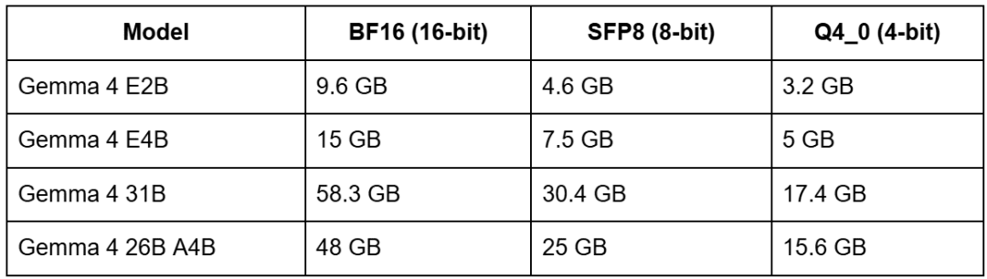
At full 16-bit precision, the 31B model needs roughly 60 GB of VRAM, which is equivalent to two A100 80GB GPUs or a single H100. But at 4-bit quantization, the same model fits in about 17 GB, which means a single RTX 4090 or A10G becomes viable.

The 26B A4B model is interesting: its full-precision footprint of 48 GB looks large, but because only 4B parameters are active during inference, it runs significantly faster than the 31B despite needing less memory. At 4-bit, it drops to 15.6 GB.

The E2B and E4B models, at 4-bit quantization, fit in 3–5 GB of VRAM, placing them in genuinely on-device territory for modern phones and edge hardware. The E suffix models are especially designed for this: their PLE (Per-Layer Embeddings) tables live in flash storage, so the actual RAM footprint is even smaller than these numbers suggest during full inference runs on mobile devices.

---

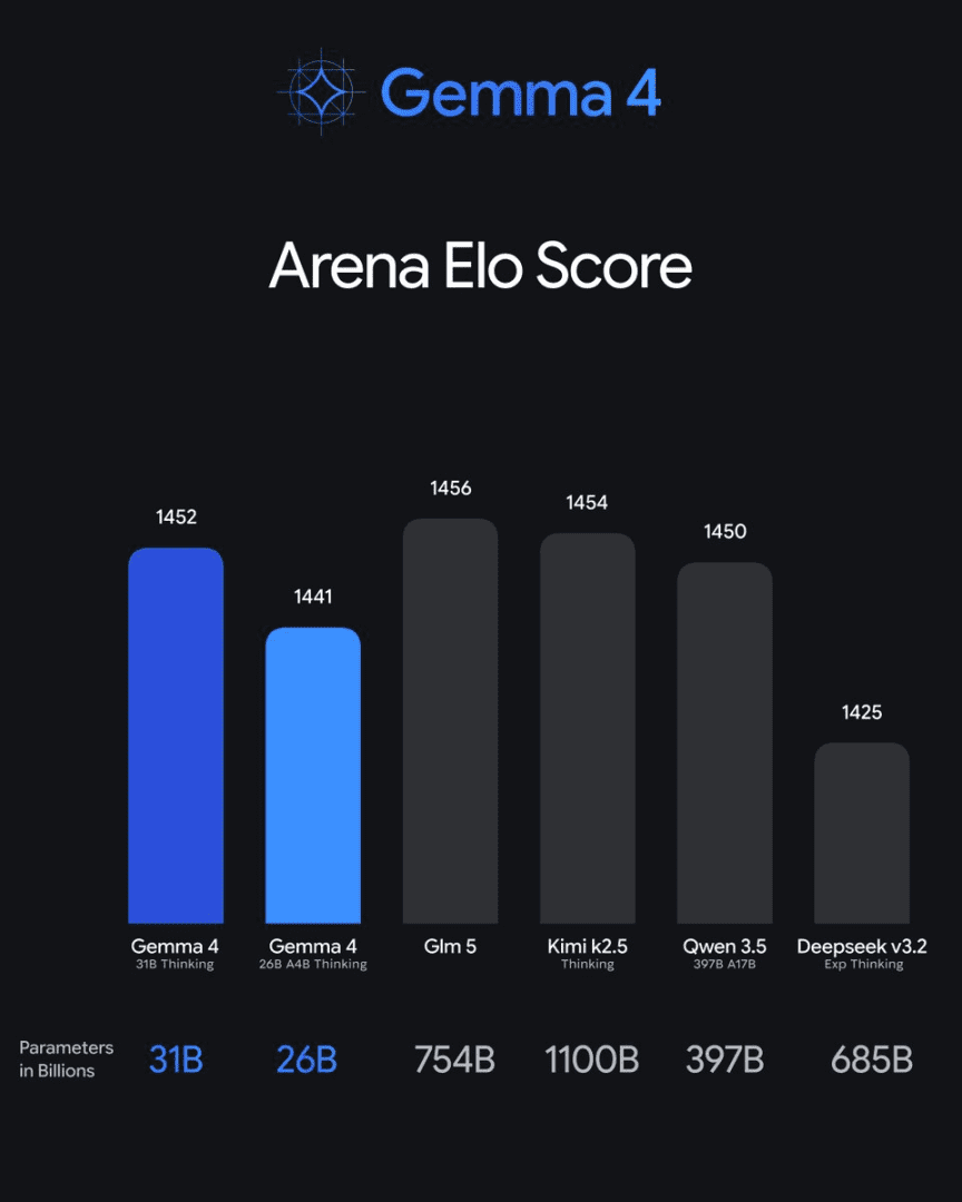
Gemma 4 Benchmarks: LMArena Elo Scores and Multimodal Performance Results

Gemma 4’s large models set a new bar for what’s achievable in the open-weight space at this parameter count.

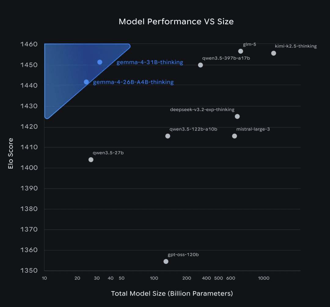
The 31B dense model achieves an estimated LMArena Elo score of 1,452 on text-only evaluations, placing it competitively with models that are significantly larger. The 26B A4B MoE model reaches 1,441, which is remarkable given that it uses only 4 billion active parameters. To put that in context: these scores are competitive with several closed-source models from mid-2024.

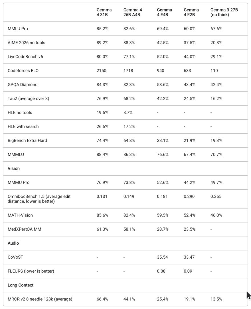
Multimodal performance follows a similar pattern. Even the vision and audio capabilities were comparable in quality to the text performance, and not degraded by the multimodal conditioning. All model sizes demonstrated strong OCR, object detection, scene description, and audio understanding.

On coding and agentic benchmarks, Gemma 4 shows notable improvements over Gemma 3, partly due to the expanded context window (128K for small models, 256K for large ones), the native function-calling support, and the thinking-mode capability.

---

How to Run Gemma 4: Transformers, llama.cpp, MLX, and Cloud Deployment Options

Google and the community have built Gemma 4 support into virtually every major inference stack. Here’s a quick summary to help you choose.

• Hugging Face Transformers: The most fully featured option for Python users. It supports all modalities, thinking mode, function calling, and the full Processor API for handling mixed text/image/audio inputs. It is the best choice for research, fine-tuning, and flexible experimentation.
• Llama.cpp: Offers highly optimized CPU and GPU inference, particularly valuable if you’re running on Apple Silicon or hardware without NVIDIA GPUs. Gemma 4 is supported in recent builds, with GGUF quantization enabling the small models to run on consumer hardware.
• MLX: The framework of choice for Apple Silicon, offering native Metal GPU acceleration. The E2B and E4B models run surprisingly fast on M-series chips via MLX, making on-Mac deployment practical.
• transformers.js: Enables in-browser inference via WebGPU. Gemma 4’s small models can run directly in a web browser (no server required), which opens up genuinely private, fully offline applications.
• Mistral.rs: A Rust-based inference engine with strong performance characteristics for production deployments.

For cloud production environments, Gemma 4 is available via the Gemini API, Google Cloud’s Vertex AI, Cloud Run, and GKE with GPU nodes. The Gemini API option is the lowest-friction path for managed serving without infrastructure work.

---

Fine-Tuning Gemma 4: LoRA, QLoRA, and TRL Training Pipeline Guide

One interesting observation from the Hugging Face team: Gemma 4 was difficult to demonstrate through fine-tuning examples because the base instruction-tuned models are already so capable. That said, fine-tuning is well-supported for domain specialization, style adaptation, or building task-specific versions.

TRL (Transformer Reinforcement Learning): The primary recommended library for supervised fine-tuning. It supports QLoRA (quantized LoRA), which dramatically reduces the memory requirements for fine-tuning, making it possible to fine-tune the 31B model on a machine with two consumer-grade GPUs if combined with 4-bit quantization. Fine-tuning is also supported on Vertex AI via TRL if you’d prefer a managed training environment.

Unsloth Studio: A no-code fine-tuning interface for users who want to adapt Gemma 4 without writing training code. It supports Gemma 4 with memory optimizations baked in.

For a full fine-tuning pipeline in code, the key is using QLoRA via Hugging Face’s peft and trl libraries, targeting the attention and feedforward projection layers. Google also provides official guides for LoRA fine-tuning via Keras, PyTorch, and the Gemma library itself.

---

Gemma 4 Prompt Formatting: Chat Templates and Multimodal Input Structure

Gemma 4 follows a specific chat template that you should be aware of when building applications. The instruction-tuned models expect input in a structured multi-turn format. When using Hugging Face Transformers, always use processor.apply_chat_template() rather than constructing prompts manually. This ensures special tokens are correctly inserted and the model receives input in the format it was trained on.

For multimodal inputs, images and audio are passed as dictionary entries alongside text in the message content list:

messages = [
    {
        "role": "user",
        "content": [
            # For image input:
            {"type": "image", "url": "https://example.com/image.png"},
            # Or for local audio:
            {"type": "audio", "path": "/path/to/audio.mp3"},
            # Text always accompanies the media:
            {"type": "text", "text": "Describe what you see/hear."},
        ],
    }
]

For video with audio (E2B and E4B only), pass load_audio_from_video=True in the apply_chat_template call. For larger models, omit this flag since they do not have an audio encoder.

---

Which Gemma 4 Model to Use: E2B vs E4B vs 26B MoE vs 31B Comparison

With 4 variants available, the choice comes down to a few key questions.

If you are building something that runs on a phone or edge device with less than 6–8 GB of RAM available for the model, the E2B or E4B are your options, and they are genuinely capable. E4B is worth the extra memory if you are doing audio-visual tasks. At 4-bit quantization, E2B runs in about 3 GB, which fits on most modern Android and iOS devices.

If you are running on a single GPU in the 16–24 GB range (RTX 3090, 4090, A10G), the 26B A4B at 4-bit quantization (15.6 GB) gives you the best intelligence-per-dollar, running at 4B-speed throughput.

If you need maximum capability and have the hardware for it (2× A100 or H100), the 31B dense model at BF16 or the 26B A4B at 16-bit precision are both strong choices. The 31B is architecturally simpler; the 26B A4B provides better throughput if you’re processing high request volumes.

If you are doing audio tasks at all, you must use E2B or E4B, since the larger models do not have an audio encoder.

---

---

Summary

Gemma 4 is best understood not as a single model but as a thoughtfully tiered family, each member engineered for a specific place in the hardware spectrum, from a smartphone to a data center GPU cluster.

The two small models (E2B and E4B) push the frontier of what is possible on-device by storing large embedding tables in flash memory rather than RAM, and by packing audio understanding alongside vision and text in a package that fits in just a few gigabytes.

The 26B A4B MoE model achieves something that still feels almost counterintuitive: the knowledge depth of a 26-billion-parameter model running at roughly the speed and cost of a 4-billion-parameter model, thanks to sparse expert routing.

The 31B dense model serves as the reliable, architecturally simple heavyweight for applications that need maximum capability without the added complexity of MoE.

Across all variants, Gemma 4 shares a core set of architectural decisions that compound in value: interleaved local-and-global attention tames the cost of long contexts; grouped query attention and the K=V cache trick shrink the memory footprint of those global layers; and pruned positional encoding keeps semantic meaning clean even across hundreds of thousands of tokens.

These are not isolated optimizations; they are a coherent strategy for squeezing frontier-level intelligence into constrained environments.

On the capability side, what sets Gemma 4 apart from prior open-weight releases is the breadth of what works out of the box. Native structured output for object detection, code generation from screenshots, audio Q&A, configurable thinking mode, and function-calling support all come without special prompting tricks or external scaffolding.

The Apache 2.0 license is a major advantage for commercial use, allowing you to deploy, modify, and build on these models without restriction.

If you take one thing away from this post, let it be this: the right way to approach Gemma 4 is not to ask “which is the best model?” but rather “what are my actual constraints — memory, latency, modality, hardware — and which variant is engineered for exactly that?”

The answer is almost certainly one of these four. The rest of this series will help you put whichever one you choose to work.

---

Citation Information

Thakur, P. “Google DeepMind’s Gemma 4: MoE, Efficiency Tricks, and Benchmarks,” PyImageSearch, S. Huot and A. Sharma, eds., 2026, https://pyimg.co/uqxzw

@incollection{Thakur_2026_google-deepminds-gemma-4-moe-efficiency-tricks-benchmarks,
  author = {Piyush Thakur},
  title = {{Google DeepMind's Gemma 4: MoE, Efficiency Tricks, and Benchmarks}},
  booktitle = {PyImageSearch},
  editor = {Susan Huot and Aditya Sharma},
  year = {2026},
  url = {https://pyimg.co/uqxzw},
}

---