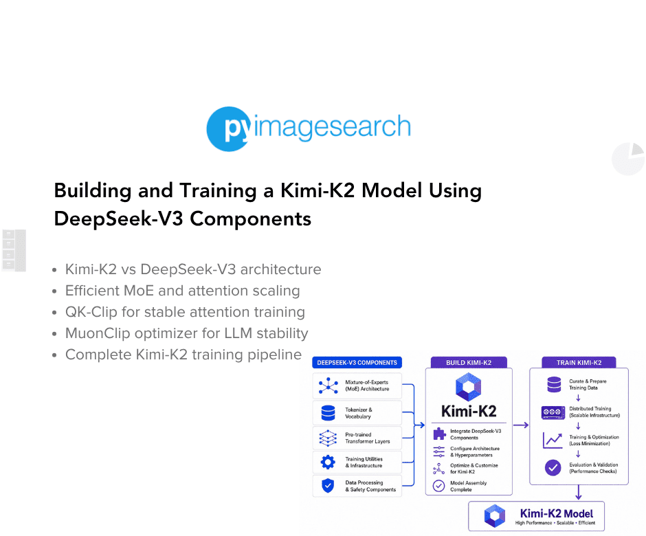
Building and Training a Kimi-K2 Model Using DeepSeek-V3 Components

The landscape of large language models (LLMs) is undergoing a fundamental transformation toward agentic intelligence, where models can autonomously perceive, plan, reason, and act within complex and dynamic environments. This paradigm shift moves beyond traditional static imitation learning toward models that actively learn through interaction, acquire skills beyond their training distribution, and adapt their behavior based on experience. Agentic intelligence represents a critical capability for the next generation of foundation models, with transformative implications for tool use, software development, and real-world autonomy.

building-training-kimi-k2-model-using-deepseek-v3-featured.png

Kimi-K2 stands at the forefront of this revolution. As a 1.04 trillion-parameter Mixture-of-Experts (MoE) language model with 32 billion activated parameters, Kimi-K2 was purposefully designed to address the core challenges of agentic capability development. The model achieves remarkable performance across diverse benchmarks:

66.1 on Tau2-bench
76.5 on ACEBench (en)
65.8 on SWE-bench Verified
53.7 on LiveCodeBench v6
75.1 on GPQA-Diamond

On the LMSYS (Large Model Systems Organization) Arena leaderboard, Kimi-K2 ranks as the top open-source model and 5th overall, competing closely with Claude 4 Opus and Claude 4 Sonnet.

In this lesson, we dive deep into the technical innovations behind Kimi-K2, focusing on its architectural differences from DeepSeek-V3, the revolutionary MuonClip optimizer, and training data improvements. We also provide a complete implementation guide using DeepSeek-V3 components as building blocks.

Kimi-K2 vs DeepSeek-V3: Key Architecture Differences in LLM Design

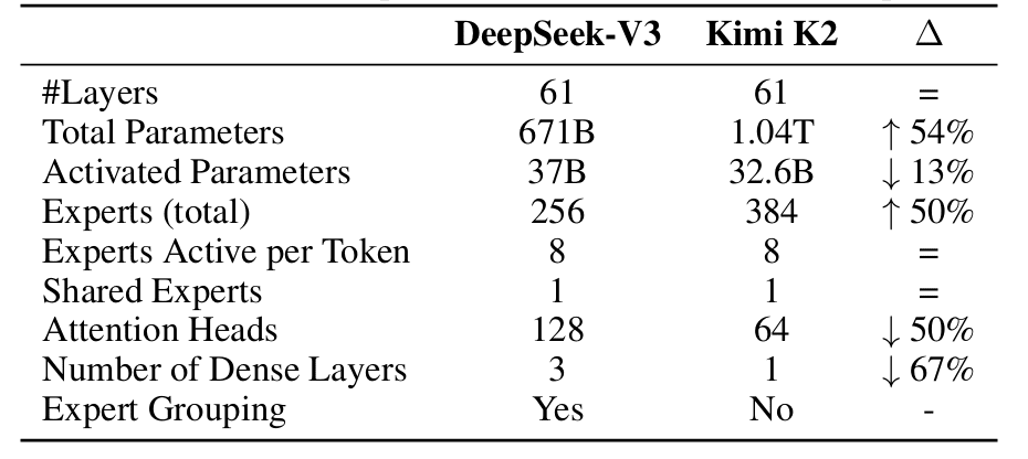
While Kimi-K2 builds on DeepSeek-V3’s architecture, several strategic modifications were made to optimize agentic capabilities and inference efficiency. Understanding these architectural differences is crucial for implementing the model effectively (Table 1).

**Table 1:** Kimi-K2 vs DeepSeek-V3 Configurations (source: Kimi Team, 2026).

Mixture of Experts Scaling in Kimi-K2: Model Size, Sparsity, and Efficiency

The most significant architectural departure lies in Kimi-K2’s aggressive sparsity scaling. Through carefully controlled small-scale experiments, the Kimi team developed a sparsity scaling law that demonstrated a clear relationship: with the number of activated parameters held constant (i.e., constant FLOPs), increasing the total number of experts consistently lowers both training and validation loss. This finding led to a dramatic increase in model sparsity.

Kimi-K2 employs 384 experts compared to DeepSeek-V3’s 256 experts, representing a 50% increase. Despite this, the model maintains 8 active experts per token, resulting in a sparsity ratio of 48 (384/8) versus DeepSeek-V3’s 32 (256/8). This increased sparsity comes with a trade-off: while total parameters grow to 1.04 trillion (54% more than DeepSeek-V3’s 671B), the number of activated parameters actually decreases to 32.6B (13% less than DeepSeek-V3’s 37B). This design choice optimizes the compute-performance frontier, achieving superior model quality while maintaining efficient inference.

Attention Head Optimization in Kimi-K2 for Efficient Long-Context LLMs

A critical optimization for agentic applications involves the number of attention heads. DeepSeek-V3 sets the number of attention heads to roughly twice the number of model layers (128 heads for 61 layers) to better utilize memory bandwidth. However, as context length increases, this design incurs significant inference overhead.

For agentic applications requiring efficient long-context processing, this becomes prohibitive. With a 128k sequence length, increasing attention heads from 64 to 128 (while keeping 384 total experts) leads to an 83% increase in inference FLOPs. Through controlled experiments, the Kimi team found that doubling the number of attention heads yields only modest improvements in validation loss (0.5% to 1.2%) under iso-token training conditions.

Given that sparsity 48 already provides strong performance, the marginal gains from doubling attention heads do not justify the inference cost. Kimi-K2 therefore uses 64 attention heads (half of DeepSeek-V3’s 128), dramatically reducing inference costs for long-context agentic workloads while maintaining competitive performance.

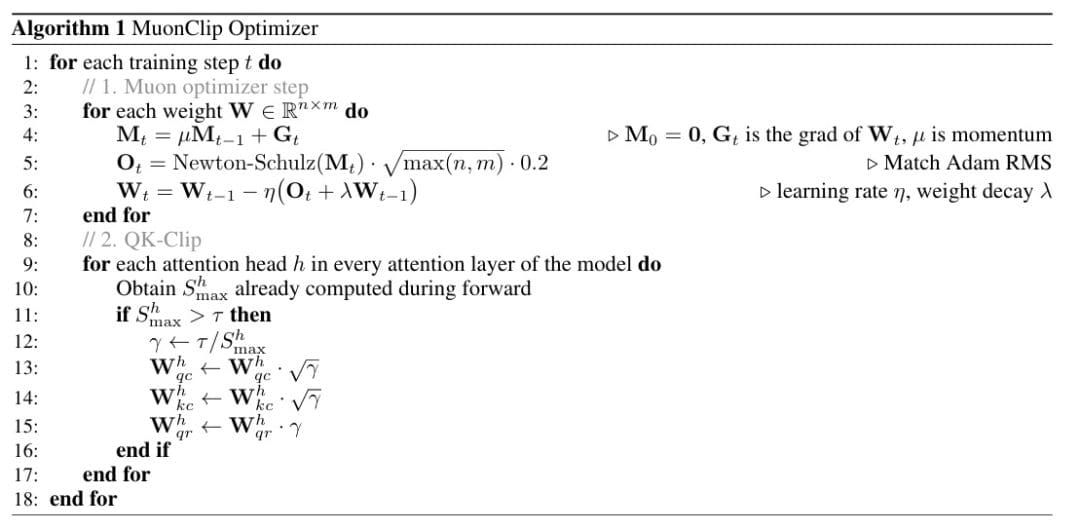
MuonClip Optimizer: Stabilizing Large-Scale LLM Training in Kimi-K2

The MuonClip optimizer represents one of the most significant innovations in Kimi-K2’s development, addressing the fundamental challenge of training stability at trillion-parameter scale while maintaining token efficiency. Understanding MuonClip requires examining both the underlying Muon optimizer and the novel QK-Clip mechanism that makes it stable for large-scale training.

Token Efficiency in LLM Training: Why It Matters for Kimi-K2

Given the increasingly limited availability of high-quality human data, token efficiency has emerged as a critical factor in LLM scaling. Token efficiency refers to how much performance improvement is achieved per token consumed during training. The Muon optimizer, introduced by Jordan et al. (2024), substantially outperforms AdamW under the same compute budget, model size, and training data volume.

Previous work in Moonlight demonstrated that Muon’s token efficiency gains make it an ideal choice for maximizing the intelligence extracted from limited high-quality tokens. However, scaling Muon to trillion-parameter models revealed a critical challenge: training instability due to exploding attention logits.

Attention Logit Explosion in LLMs: Training Instability and Challenges

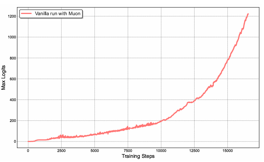
During medium-scale training runs using vanilla Muon, attention logits rapidly exceeded magnitudes of 1000, leading to numerical instabilities and occasional training divergence (Figure 1). This phenomenon occurred more frequently with Muon than with AdamW, suggesting that Muon’s aggressive optimization dynamics amplify instabilities in the attention mechanism.

**Figure 1:** Attention logits rapidly exceed 1000, which could lead to potential numerical instabilities and even training divergence (source: Kimi Team, 2026).

Existing mitigation strategies proved insufficient:

Logit soft-capping (used in Gemma) directly clips attention logits, but the dot products between queries and keys can still grow excessively before capping is applied
Query-Key Normalization (QK-Norm) (Dehghani et al., 2023) is incompatible with Multi-head Latent Attention (MLA) because full key matrices are not explicitly materialized during inference

QK-Clip: Preventing Attention Logit Explosion in Kimi-K2 Training

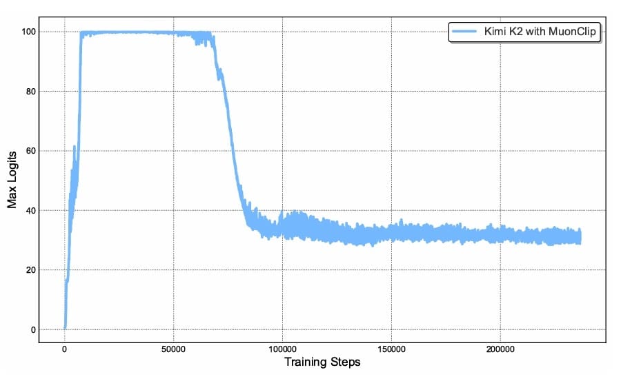
To address this fundamental challenge, the Kimi team proposed QK-Clip, a novel weight-clipping mechanism that explicitly constrains attention logits by rescaling the query and key projection weights post-update. The elegance of QK-Clip lies in its simplicity: it does not alter forward and backward computation in the current step but instead uses maximum logits as a guiding signal to control weight growth (Figure 2).

**Figure 2:** Maximum logits for Kimi-K2 with MuonClip and τ = 100 over the entire training run. The max logits rapidly increase to the capped value of 100 before decaying to a stable range (source: Kimi Team, 2026).

For each attention head $h$ , the attention mechanism computes:

$Q^h = X W_q^h, \quad K^h = X W_k^h, \quad V^h = X W_v^h$

The attention output is:

$O^h = \text{softmax}\left(\dfrac{1}{\sqrt{d}} Q^h (K^h)^\top\right) V^h$

QK-Clip defines the max logit per head as:

$S_{\max}^h = \dfrac{1}{\sqrt{d}} \max_{X \in B} \max_{i,j} Q_i^h (K_j^h)^\top$

where $B$ is the current batch and $i, j$ index different tokens.

When $S_{\max}^h$ exceeds a threshold $\tau$ (set to 100 for Kimi-K2), QK-Clip rescales the weights. Critically, the rescaling is applied per-head rather than globally, minimizing intervention on heads that remain stable:

$\gamma_h = \min(1, \tau / S_{\max}^h)$ .

This per-head, component-aware clipping represents a substantial refinement over naive global clipping strategies.

Figure 3 describes the complete algorithm for MuonClip Optimizer.

**Figure 3:** MuonClip Algorithm (source: Kimi Team, 2026).

Training Data Optimization for Kimi-K2: Improving Token Utility in LLMs

Beyond architectural and optimizer innovations, Kimi-K2’s superior performance stems significantly from strategic improvements in training data. With high-quality human-generated data becoming increasingly scarce, the focus shifts to increasing token utility, defined as the effective learning signal each token contributes to model updates.

Token Utility in LLM Training: Maximizing Learning per Token

Token efficiency in pre-training encompasses 2 related but distinct concepts:

Optimizer efficiency: How effectively the optimizer extracts signal from each gradient update (addressed by MuonClip)
Token utility: The inherent information density and learning signal in each token

Increasing token utility directly improves token efficiency. A naive approach involves repeated exposure to the same tokens across multiple epochs, but this leads to overfitting and reduced generalization. The key innovation in Kimi-K2 lies in a sophisticated synthetic data generation strategy that amplifies high-quality tokens without inducing overfitting.

Knowledge Data Rephrasing for LLMs: Improving Training Data Quality

Pre-training on knowledge-intensive text presents a fundamental trade-off: a single epoch is insufficient for comprehensive knowledge absorption, while multi-epoch repetition yields diminishing returns. To resolve this tension, Kimi-K2 employs a synthetic rephrasing framework with the following 3 key components.

Style- and Perspective-Diverse Prompting

To enhance linguistic diversity while maintaining factual integrity, carefully engineered prompts guide a large language model to generate faithful rephrasings in varied styles and perspectives. This approach ensures that while surface-level linguistic features change, the underlying factual content remains consistent. The diversity of expressions forces the model to learn robust representations of the same knowledge across multiple linguistic realizations.

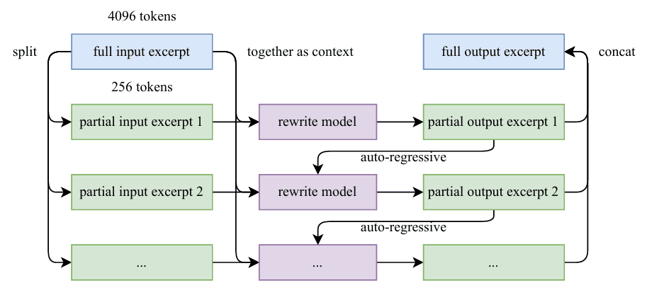
Chunk-wise Autoregressive Generation

Long documents pose a challenge for standard LLM-based rewriting due to implicit output length limitations. Kimi-K2 addresses this through a chunk-based autoregressive strategy: documents are segmented, each segment is rephrased individually with preserved context, and segments are stitched back together to form complete passages. This methodology prevents information loss and maintains global coherence across extended texts (Figure 4).

Fidelity Verification

To ensure consistency between original and rewritten content, fidelity checks compare the semantic alignment of each rephrased passage with its source. This quality control step prevents the introduction of hallucinations or factual errors during the rephrasing process.

**Figure 4:** Auto-regressive chunk-wise rephrasing pipeline for long input excerpts (source: Kimi Team, 2026).

Mathematics Data Rephrasing

To enhance mathematical reasoning capabilities, high-quality mathematical documents are rewritten into a “learning-note” style following SwallowMath methodology (Figure 5). This transformation converts dense mathematical exposition into more pedagogical formats that better support learning. Additionally, data diversity is increased through the translation of high-quality mathematical materials from other languages into English, effectively multiplying the available high-quality mathematical training data.

**Figure 5:** Four-stage pipeline for constructing SwallowMath (source: Fujii et al., 2026).

Overall Pre-training Corpus

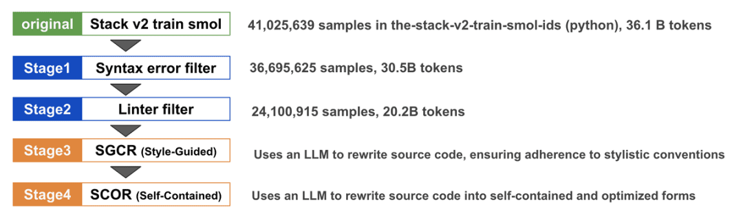
The complete Kimi-K2 pre-training corpus comprises 15.5 trillion tokens of curated, high-quality data spanning 4 primary domains:

Web Text: General knowledge and natural language understanding
Code: Programming and structured reasoning
Mathematics: Quantitative reasoning and formal problem-solving
Knowledge: Domain-specific expertise and factual information

Kimi-K2 Implementation: Training an Open-Source LLM with DeepSeek-V3

In this section, we walk through the key implementation details for training Kimi-K2, focusing specifically on the components that differ from the standard DeepSeek-V3 implementation. We’ll examine the enhanced Multi-head Latent Attention with max logit tracking, the MuonClip optimizer implementation, and the custom training setup.

Multi-Head Latent Attention (MLA) with Max Logit Tracking in Kimi-K2

The Multi-head Latent Attention (MLA) mechanism in Kimi-K2 extends DeepSeek-V3’s implementation with critical modifications to support QK-Clip. The key enhancement is per-head max-logit tracking during the forward pass, which provides the signal needed for weight clipping by the optimizer.

class MultiheadLatentAttention(nn.Module):
    
    def __init__(self, config: DeepSeekConfig):
        super().__init__()
        self.config = config
        self.n_embd = config.n_embd
        self.n_head = config.n_head
        self.head_dim = config.n_embd // config.n_head

        # Compression dimensions
        self.kv_lora_rank = config.kv_lora_rank
        self.q_lora_rank = config.q_lora_rank
        self.rope_dim = config.rope_dim

        # KV compression
        self.kv_proj = nn.Linear(self.n_embd, self.kv_lora_rank, bias=False)
        self.kv_norm = RMSNorm(self.kv_lora_rank)

        # KV decompression
        self.k_decompress = nn.Linear(self.kv_lora_rank, self.n_head * self.head_dim, bias=False)
        self.v_decompress = nn.Linear(self.kv_lora_rank, self.n_head * self.head_dim, bias=False)

        # Query compression
        self.q_proj = nn.Linear(self.n_embd, self.q_lora_rank, bias=False)
        self.q_decompress = nn.Linear(self.q_lora_rank, self.n_head * self.head_dim, bias=False)

        # RoPE projections
        self.k_rope_proj = nn.Linear(self.n_embd, self.n_head * self.rope_dim, bias=False)
        self.q_rope_proj = nn.Linear(self.q_lora_rank, self.n_head * self.rope_dim, bias=False)

        # Output projection
        self.o_proj = nn.Linear(self.n_head * self.head_dim, self.n_embd, bias=config.bias)

        # Dropout
        self.attn_dropout = nn.Dropout(config.dropout)
        self.resid_dropout = nn.Dropout(config.dropout)

        # RoPE
        self.rope = RotaryEmbedding(self.rope_dim, config.block_size)

        # Causal mask
        self.register_buffer(
            "causal_mask",
            torch.tril(torch.ones(config.block_size, config.block_size)).view(
                1, 1, config.block_size, config.block_size
            )
        )

        self.max_logits = 0.0  # Track maximum attention logits

On Lines 1-47, we define the MLA architecture following DeepSeek-V3’s design with compression and decompression of queries and key-values through low-rank projections. The key innovation appears on Line 49, where we initialize self.max_logits = 0.0, a critical state variable that tracks the maximum attention logits across heads. This tracking mechanism is essential for QK-Clip to function properly.

    def forward(self, x: torch.Tensor, attention_mask: Optional[torch.Tensor] = None):
        B, T, C = x.size()

        # Compression phase
        kv_compressed = self.kv_norm(self.kv_proj(x))
        q_compressed = self.q_proj(x)

        # Decompression phase
        k_content = self.k_decompress(kv_compressed)
        v = self.v_decompress(kv_compressed)
        q_content = self.q_decompress(q_compressed)

        # RoPE components
        k_rope = self.k_rope_proj(x)
        q_rope = self.q_rope_proj(q_compressed)

        # Reshape for multi-head attention
        k_content = k_content.view(B, T, self.n_head, self.head_dim).transpose(1, 2)
        v = v.view(B, T, self.n_head, self.head_dim).transpose(1, 2)
        q_content = q_content.view(B, T, self.n_head, self.head_dim).transpose(1, 2)
        k_rope = k_rope.view(B, T, self.n_head, self.rope_dim).transpose(1, 2)
        q_rope = q_rope.view(B, T, self.n_head, self.rope_dim).transpose(1, 2)

        # Apply RoPE
        cos, sin = self.rope(x, T)
        q_rope = apply_rope(q_rope, cos, sin)
        k_rope = apply_rope(k_rope, cos, sin)

        # Concatenate content and rope parts
        q = torch.cat([q_content, q_rope], dim=-1)
        k = torch.cat([k_content, k_rope], dim=-1)

On Lines 52-82, we implement the standard forward pass through the compression-decompression pipeline. The input undergoes compression via kv_proj and q_proj, followed by decompression through dedicated linear layers. We then reshape tensors for multi-head processing and apply Rotary Position Embeddings (RoPE) separately to content and positional components. This separation allows per-head QK-Clip to target only the appropriate components without affecting shared rotary embeddings.

        # Concatenate content and rope parts
        q = torch.cat([q_content, q_rope], dim=-1)
        k = torch.cat([k_content, k_rope], dim=-1)

        # Attention computation
        scale = 1.0 / math.sqrt(q.size(-1))
        scores = torch.matmul(q, k.transpose(-2, -1)) * scale

        with torch.no_grad():
            # self.max_logits = torch.max(scores, dim=1).item()
            self.max_logits = list(torch.max(scores.transpose(1, 0).contiguous().view(scores.shape[1], -1), dim=-1)[0])

        # Apply causal mask
        scores = scores.masked_fill(self.causal_mask[:, :, :T, :T] == 0, float('-inf'))

        # Apply padding mask if provided
        if attention_mask is not None:
            padding_mask_additive = (1 - attention_mask).unsqueeze(1).unsqueeze(2) * float('-inf')
            scores = scores + padding_mask_additive

        # Softmax and dropout
        attn_weights = F.softmax(scores, dim=-1)
        attn_weights = self.attn_dropout(attn_weights)

        # Apply attention to values
        out = torch.matmul(attn_weights, v)

        # Reshape and project
        out = out.transpose(1, 2).contiguous().view(B, T, self.n_head * self.head_dim)
        out = self.resid_dropout(self.o_proj(out))

        return out

On Lines 89-94, we compute attention scores and implement the crucial max logit tracking. The score computation follows standard scaled dot-product attention. However, Lines 92-94 represent a key departure from vanilla DeepSeek-V3: we track the maximum attention logit per head using torch.no_grad() to avoid affecting gradients. The scores tensor has shape [batch, num_heads, seq_len, seq_len], and we transpose and reshape to extract per-head maximum values. This per-head granularity enables targeted intervention only on heads exhibiting logit explosion, minimizing disruption to stable heads.

On Lines 97-113, we complete the attention mechanism with causal masking, optional padding masks, softmax normalization, and dropout. The final output projection maintains the standard MLA architecture. The elegance of this implementation lies in its non-invasiveness: max logit tracking adds minimal computational overhead (a single max operation under torch.no_grad) while providing the critical signal for optimizer-level weight clipping.

Implementing the MuonClip Optimizer for Stable LLM Training

The MuonClip optimizer represents the core innovation enabling stable trillion-parameter training. Our implementation integrates Newton-Schulz orthogonalization, RMS matching, weight decay, and per-head QK-Clip into a unified optimizer.

def apply_qk_clip_per_head(
    query_weights: torch.Tensor,
    key_weights: torch.Tensor,
    max_logits_per_head: Union[List[float], torch.Tensor],
    tau: float = 100.0
) -> None:
        if isinstance(max_logits_per_head, list):
        max_logits_per_head = torch.tensor(
            max_logits_per_head,
            device=query_weights.device,
            dtype=query_weights.dtype
        )
    apply_qk_clip_vectorized(query_weights, key_weights, max_logits_per_head, tau)

On Lines 1-13, we define the entry point for the QK-Clip application. The function accepts query and key projection weights along with per-head max logits and a threshold $\tau$ (defaulting to 100). We handle both list and tensor inputs for flexibility, converting lists to tensors on the appropriate device with matching dtype. The critical design choice here is in-place modification: we directly modify weight tensors to avoid memory allocation overhead during optimization.

def apply_qk_clip_per_head(
    query_weights: torch.Tensor,
    key_weights: torch.Tensor,
    max_logits_per_head: Union[List[float], torch.Tensor],
    tau: float = 100.0
) -> None:
        if isinstance(max_logits_per_head, list):
        max_logits_per_head = torch.tensor(
            max_logits_per_head,
            device=query_weights.device,
            dtype=query_weights.dtype
        )
    apply_qk_clip_vectorized(query_weights, key_weights, max_logits_per_head, tau)

@torch.no_grad()
def apply_qk_clip_vectorized(
    query_weights: torch.Tensor,
    key_weights: torch.Tensor,
    max_logits_per_head: torch.Tensor,
    tau: float = 100.0
) -> None:
    
    q_out, q_in = query_weights.shape[0], query_weights.shape[1]
    k_out, k_in = key_weights.shape[0], key_weights.shape[1]
    num_heads = len(max_logits_per_head)
    d_k = q_out // num_heads

    # Ensure tensor type
    if not isinstance(max_logits_per_head, torch.Tensor):
        max_logits_per_head = torch.tensor(
            max_logits_per_head,
            device=query_weights.device,
            dtype=query_weights.dtype
        )

    # Compute scaling factors: gamma = tau / max_logit where max_logit > tau
    needs_clip = max_logits_per_head > tau

On Lines 15-48, we extract dimensions and ensure tensor type compatibility. We first extract dimensions and compute the per-head scaling factor $\gamma_h = \min(1, \tau / S_{\max}^h)$ only for heads where $S_{\max}^h > \tau$ .

@torch.no_grad()
def apply_qk_clip_vectorized(
    query_weights: torch.Tensor,
    key_weights: torch.Tensor,
    max_logits_per_head: torch.Tensor,
    tau: float = 100.0
) -> None:
    
    q_out, q_in = query_weights.shape[0], query_weights.shape[1]
    k_out, k_in = key_weights.shape[0], key_weights.shape[1]
    num_heads = len(max_logits_per_head)
    d_k = q_out // num_heads

    # Ensure tensor type
    if not isinstance(max_logits_per_head, torch.Tensor):
        max_logits_per_head = torch.tensor(
            max_logits_per_head,
            device=query_weights.device,
            dtype=query_weights.dtype
        )

    # Compute scaling factors: gamma = tau / max_logit where max_logit > tau
    needs_clip = max_logits_per_head > tau

    # If no clipping needed, return early
    if not needs_clip.any():
        return

    gamma = torch.where(
        needs_clip,
        tau / max_logits_per_head.clamp(min=1e-8),
        torch.ones_like(max_logits_per_head)
    )
    sqrt_gamma = torch.sqrt(gamma)

    # Reshape weights to [d_model, num_heads, d_k] for per-head scaling
    # Views share underlying storage, so in-place ops modify original tensor
    q_reshaped = query_weights.view(q_out // num_heads, num_heads, q_in)
    k_reshaped = key_weights.view(k_out // num_heads, num_heads, k_in)

    # Apply per-head scaling IN-PLACE: broadcast sqrt_gamma [num_heads] over [d_model, num_heads, d_k]
    q_reshaped.mul_(sqrt_gamma.view(1, num_heads, 1))
    k_reshaped.mul_(sqrt_gamma.view(1, num_heads, 1))

    q_reshaped = q_reshaped.view(q_out, q_in)
    k_reshaped = k_reshaped.view(k_out, k_in)

On Lines 52-60, we restart the function definition and extract dimensions. On Lines 80-97, we perform the actual weight clipping through careful tensor reshaping and in-place multiplication. The weights are reshaped from [d_model, d_model] to [d_model/num_heads, num_heads, d_k] to expose the head dimension. We then apply $\sqrt{\gamma_h}$ scaling using in-place multiplication (mul_) with broadcasting. The square root scaling ensures that when query and key both receive $\sqrt{\gamma}$ , their dot product receives the full $\gamma$ scaling. This elegant mathematical property allows us to clip attention logits by rescaling the weights that produce them, rather than clipping logits directly after they’re computed.

Lines 77 and 78 implement early exit if no head requires clipping, which becomes a common case later in training when attention logits stabilize. This optimization avoids unnecessary computation when the model is well-behaved.

class MuonClip(torch.optim.Optimizer):
    def __init__(
        self,
        params,
        lr: float = 1e-3,
        momentum: float = 0.95,
        weight_decay: float = 0.01,
        tau: float = 100.0,
        ns_steps: int = 5,
        eps: float = 1e-7
    ):
        if lr < 0.0:
            raise ValueError(f"Invalid learning rate: {lr}")
        if not 0.0 <= momentum <= 1.0:
            raise ValueError(f"Invalid momentum value: {momentum}")
        if weight_decay < 0.0:
            raise ValueError(f"Invalid weight_decay value: {weight_decay}")
        if tau <= 0.0:
            raise ValueError(f"Invalid tau value: {tau}")

        defaults = dict(
            lr=lr,
            momentum=momentum,
            weight_decay=weight_decay,
            tau=tau,
            ns_steps=ns_steps,
            eps=eps
        )
        super().__init__(params, defaults)

        # For QK-Clip functionality
        self.model = None
        self.attention_layers = []

    def set_model(self, model: nn.Module):
        self.model = model
        if hasattr(model, 'get_attention_layers'):
            self.attention_layers = model.get_attention_layers()

On Lines 1-33, we define the MuonClip optimizer class, inheriting from PyTorch’s base Optimizer. The constructor accepts standard hyperparameters (learning rate, momentum, weight decay) plus QK-Clip-specific parameters ( $\tau$ and Newton-Schulz steps). We validate all parameters and initialize state tracking. Critically, Lines 35-38 implement model registration through set_model(), which extracts attention layers for later QK-Clip application. This design separates optimizer logic from model architecture, allowing the optimizer to operate on any model exposing a get_attention_layers() method.

    @torch.no_grad()
    def step(self, closure: Optional[Callable] = None) -> Optional[float]:
        loss = None
        if closure is not None:
            with torch.enable_grad():
                loss = closure()

        for group in self.param_groups:
            lr = group['lr']
            momentum = group['momentum']
            weight_decay = group['weight_decay']
            ns_steps = group['ns_steps']
            eps = group['eps']

            for p in group['params']:
                if p.grad is None:
                    continue

                grad = p.grad
                state = self.state[p]

                # Initialize momentum buffer
                if len(state) == 0:
                    state['momentum_buffer'] = torch.zeros_like(p)

                buf = state['momentum_buffer']

                # Apply momentum: Mt = μMt−1 + Gt
                buf.mul_(momentum).add_(grad)

                if p.ndim >= 2:  # 2D+ parameters - use Muon
                    # Apply Newton-Schulz orthogonalization
                    if p.ndim > 2:
                        original_shape = buf.shape
                        buf_2d = buf.view(buf.shape[0], -1)
                        orthogonal_update = newton_schulz(buf_2d, ns_steps, eps)
                        orthogonal_update = orthogonal_update.view(original_shape)
                    else:
                        orthogonal_update = newton_schulz(buf, ns_steps, eps)

                    # RMS matching factor: √(max(n,m) × 0.2)
                    n, m = p.shape[0], p.shape[1] if p.ndim > 1 else 1
                    rms_factor = math.sqrt(max(n, m) * 0.2)
                    orthogonal_update = orthogonal_update * rms_factor

                    # Update: Wt = Wt−1 − η(Ot + λWt−1)
                    p.add_(orthogonal_update + weight_decay * p, alpha=-lr)
                else:
                    # 1D parameters - standard momentum
                    p.add_(buf + weight_decay * p, alpha=-lr)

        # Apply QK-Clip
        self._apply_qk_clip()

        return loss

On Lines 41-94, we implement the core optimization step integrating Muon updates with QK-Clip. The step begins with standard closure handling and parameter group iteration. Lines 41-68 implement momentum accumulation ( $M_t = \mu M_{t-1} + G_t$ ) using in-place operations for memory efficiency. The critical branching occurs at Line 70: parameters with 2+ dimensions receive Muon treatment.

On Lines 72-83, we apply the Muon update for matrix parameters. Newton-Schulz orthogonalization produces an orthogonal approximation of the momentum buffer, which we then scale by $\sqrt{\max(n,m)} \times 0.2$ to match AdamW’s RMS characteristics. This scaling ensures Muon’s updates have similar magnitudes to AdamW, enabling easier hyperparameter transfer. Finally, Line 86 applies the update with weight decay: $W_t = W_{t-1} - \eta(O_t + \lambda W_{t-1})$ . Line 89 applies standard momentum updates to 1D parameters such as biases and normalization layers.

    def _apply_qk_clip(self):
        """Apply QK-Clip to attention layers to prevent logit explosion."""
        if not self.attention_layers:
            return

        tau = self.param_groups[0]['tau']

        for attention_layer in self.attention_layers:
            if not hasattr(attention_layer, 'max_logits'):
                continue

            max_logits = attention_layer.max_logits
            if not max_logits:
                continue


            # Handle both scalar and per-head max logits
            if isinstance(max_logits, (int, float)):
                max_logits = [max_logits]


            apply_qk_clip_per_head(
                    attention_layer.k_decompress.weight.data,
                    attention_layer.q_decompress.weight.data,
                    max_logits,
                    tau
            )

On Lines 96-122, we apply QK-Clip after all weight updates. The _apply_qk_clip() method iterates through all registered attention layers, extracts their max_logits attribute (populated during forward pass), and applies per-head clipping to the query and key decompression weights. This post-update clipping ensures weights don’t grow unboundedly across training steps while preserving gradient information within each step.

Complete Kimi-K2 Training Pipeline: Setup, Config, and Optimization

Finally, we bring everything together in a complete training configuration:

config = DeepSeekConfig()
config.multi_token_predict = 0
config.n_experts = 8
config.n_head = 4

training_args = TrainingArguments(
    output_dir="./kimik2_checkpoints",
    num_train_epochs=2,
    per_device_train_batch_size=8,
    per_device_eval_batch_size=4,
    learning_rate=5e-4,
    warmup_steps=10,
    weight_decay=0.01,
    logging_dir="./kimik2_checkpoints/logs",
    logging_steps=50,
    save_steps=50,
    save_total_limit=3,
    eval_steps=50,
    eval_strategy="steps",
    save_strategy="steps",
    metric_for_best_model="eval_loss",
    greater_is_better=False,
    gradient_accumulation_steps=4,
    fp16=True,
    dataloader_num_workers=2,
    remove_unused_columns=False,
    report_to="none",
    push_to_hub=False,
    save_safetensors=False,
)

On Lines 1-4, we configure the model architecture. Kimi-K2 does not use Multi-Token Prediction, so we disable multi-token prediction (multi_token_predict=0) to simplify training and focus on core capabilities. We use 8 experts for this educational implementation rather than the hundreds used in production-scale Kimi-K2 and DeepSeek-V3 models. We also use 4 attention heads for this small-scale educational implementation, compared to the production-scale configurations used in DeepSeek-V3 and Kimi-K2.

On Lines 6-30, we define training arguments following best practices for small-scale experiments. We use gradient accumulation (4 steps) to simulate larger batch sizes with limited GPU memory, enable mixed-precision training (fp16=True) for speed and memory efficiency, and configure regular evaluation and checkpointing every 50 steps. The learning rate of 5e-4 is conservative for stable training, with a brief 10-step warmup.

model = DeepSeek(config)

data_collator = DeepSeekDataCollator(tokenizer)

optimizer = MuonClip(model.parameters(), lr=5e-3)
optimizer.set_model(model)

# Create trainer
trainer = DeepSeekTrainer(
    model=model,
    args=training_args,
    train_dataset=train_dataset,
    eval_dataset=eval_dataset,
    data_collator=data_collator,
    optimizers=(optimizer, None)
)

print("✓ Trainer created. Starting training...")
print("=" * 80)

# Train!
trainer.train()

print("=" * 80)
print("✓ Training complete!")

# Save final model
trainer.save_model("./kimik2_final")
tokenizer.save_pretrained("./kimik2_final")
print("✓ Model saved to ./kimik2_final")

On Lines 31-36, we initialize the model and create a MuonClip optimizer. Critically, Line 36 registers the model with the optimizer using set_model(), enabling QK-Clip to access attention layers. This registration must occur before training begins.

On Lines 39-60, we instantiate the custom trainer with all components and launch training. The optimizers=(optimizer, None) argument provides our custom optimizer to Hugging Face Trainer, overriding its default optimizer creation. After training completes, we save both the model weights and tokenizer for later inference.

What's next? We recommend PyImageSearch University.

Course information:
86+ total classes • 115+ hours hours of on-demand code walkthrough videos • Last updated: May 2026
★★★★★ 4.84 (128 Ratings) • 16,000+ Students Enrolled

I strongly believe that if you had the right teacher you could master computer vision and deep learning.

Do you think learning computer vision and deep learning has to be time-consuming, overwhelming, and complicated? Or has to involve complex mathematics and equations? Or requires a degree in computer science?

That’s not the case.

All you need to master computer vision and deep learning is for someone to explain things to you in simple, intuitive terms. And that’s exactly what I do. My mission is to change education and how complex Artificial Intelligence topics are taught.

If you're serious about learning computer vision, your next stop should be PyImageSearch University, the most comprehensive computer vision, deep learning, and OpenCV course online today. Here you’ll learn how to successfully and confidently apply computer vision to your work, research, and projects. Join me in computer vision mastery.

Inside PyImageSearch University you'll find:

✓ 86+ courses on essential computer vision, deep learning, and OpenCV topics
✓ 86 Certificates of Completion
✓ 115+ hours hours of on-demand video
✓ Brand new courses released regularly, ensuring you can keep up with state-of-the-art techniques
✓ Pre-configured Jupyter Notebooks in Google Colab
✓ Run all code examples in your web browser — works on Windows, macOS, and Linux (no dev environment configuration required!)
✓ Access to centralized code repos for all 540+ tutorials on PyImageSearch
✓ Easy one-click downloads for code, datasets, pre-trained models, etc.
✓ Access on mobile, laptop, desktop, etc.

Click here to join PyImageSearch University

Summary

We began by detailing how to train Kimi-K2 from scratch using DeepSeek-V3 components, emphasizing the architectural differences that set Kimi-K2 apart. We explored the model’s scale and sparsity, showing that reducing the number of attention heads allowed us to balance efficiency and performance. A key part of this journey was the introduction of the MuonClip optimizer, which stabilizes training while pushing the limits of large-scale language modeling.

We then turned to the challenges of token efficiency and the attention logit explosion problem. To address these, we introduced the QK-Clip innovation, which helped us control runaway logits and improve overall stability. Alongside this, we refined our training data pipeline, focusing on token utility and knowledge data rephrasing to ensure that every token contributed meaningfully to the model’s learning process. These improvements allowed us to maximize the value of the data while keeping training efficient.

Finally, we described the implementation details, including enhanced multi-head latent attention with max logit tracking and the practical integration of the MuonClip optimizer. We concluded with a complete training setup, showing how all these innovations came together to make Kimi-K2 a robust, efficient, and scalable model. By combining architectural refinements, optimizer breakthroughs, and data improvements, this lesson demonstrated how these techniques push the boundaries of what’s possible in modern language model training.

Citation Information

Mangla, P. “Building and Training a Kimi-K2 Model Using DeepSeek-V3 Components,” PyImageSearch, S. Huot, A. Sharma, and P. Thakur, eds., 2026, https://pyimg.co/d3tge

@incollection{Mangla_2026_building-training-kimi-k2-model-using-deepseek-v3,
  author = {Puneet Mangla},
  title = {{Building and Training a Kimi-K2 Model Using DeepSeek-V3 Components}},
  booktitle = {PyImageSearch},
  editor = {Susan Huot and Aditya Sharma and Piyush Thakur},
  year = {2026},
  url = {https://pyimg.co/d3tge},
}

To download the source code to this post (and be notified when future tutorials are published here on PyImageSearch), simply enter your email address in the form below!

Download the Source Code and FREE 17-page Resource Guide

Enter your email address below to get a .zip of the code and a FREE 17-page Resource Guide on Computer Vision, OpenCV, and Deep Learning. Inside you'll find my hand-picked tutorials, books, courses, and libraries to help you master CV and DL!