OpenCV panorama stitching

In today’s blog post, I’ll demonstrate how to perform image stitching and panorama construction using Python and OpenCV. Given two images, we’ll “stitch” them together to create a simple panorama, as seen in the example above.

To construct our image panorama, we’ll utilize computer vision and image processing techniques such as: keypoint detection and local invariant descriptors; keypoint matching; RANSAC; and perspective warping.

Since there are major differences in how OpenCV 2.4.X and OpenCV 3.X handle keypoint detection and local invariant descriptors (such as SIFT and SURF), I’ve taken special care to provide code that is compatible with both versions (provided that you compiled OpenCV 3 with opencv_contrib support, of course).

In future blog posts we’ll extend our panorama stitching code to work with multiple images rather than just two.

Read on to find out how panorama stitching with OpenCV is done.

OpenCV panorama stitching

Our panorama stitching algorithm consists of four steps:

• Step #1: Detect keypoints (DoG, Harris, etc.) and extract local invariant descriptors (SIFT, SURF, etc.) from the two input images.
• Step #2: Match the descriptors between the two images.
• Step #3: Use the RANSAC algorithm to estimate a homography matrix using our matched feature vectors.
• Step #4: Apply a warping transformation using the homography matrix obtained from Step #3.

We’ll encapsulate all four of these steps inside panorama.py , where we’ll define a Stitcher class used to construct our panoramas.

The Stitcher class will rely on the imutils Python package, so if you don’t already have it installed on your system, you’ll want to go ahead and do that now:

$ pip install imutils

Let’s go ahead and get started by reviewing panorama.py :

# import the necessary packages
import numpy as np
import imutils
import cv2

class Stitcher:
	def __init__(self):
		# determine if we are using OpenCV v3.X
		self.isv3 = imutils.is_cv3(or_better=True)

We start off on Lines 2-4 by importing our necessary packages. We’ll be using NumPy for matrix/array operations, imutils for a set of OpenCV convenience methods, and finally cv2 for our OpenCV bindings.

From there, we define the Stitcher class on Line 6. The constructor to Stitcher simply checks which version of OpenCV we are using by making a call to the is_cv3 method. Since there are major differences in how OpenCV 2.4 and OpenCV 3 handle keypoint detection and local invariant descriptors, it’s important that we determine the version of OpenCV that we are using.

Next up, let’s start working on the stitch method:

	def stitch(self, images, ratio=0.75, reprojThresh=4.0,
		showMatches=False):
		# unpack the images, then detect keypoints and extract
		# local invariant descriptors from them
		(imageB, imageA) = images
		(kpsA, featuresA) = self.detectAndDescribe(imageA)
		(kpsB, featuresB) = self.detectAndDescribe(imageB)

		# match features between the two images
		M = self.matchKeypoints(kpsA, kpsB,
			featuresA, featuresB, ratio, reprojThresh)

		# if the match is None, then there aren't enough matched
		# keypoints to create a panorama
		if M is None:
			return None

The stitch method requires only a single parameter, images , which is the list of (two) images that we are going to stitch together to form the panorama.

We can also optionally supply ratio , used for David Lowe’s ratio test when matching features (more on this ratio test later in the tutorial), reprojThresh which is the maximum pixel “wiggle room” allowed by the RANSAC algorithm, and finally showMatches , a boolean used to indicate if the keypoint matches should be visualized or not.

Line 15 unpacks the images list (which again, we presume to contain only two images). The ordering to the images list is important: we expect images to be supplied in left-to-right order. If images are not supplied in this order, then our code will still run — but our output panorama will only contain one image, not both.

Once we have unpacked the images list, we make a call to the detectAndDescribe method on Lines 16 and 17. This method simply detects keypoints and extracts local invariant descriptors (i.e., SIFT) from the two images.

Given the keypoints and features, we use matchKeypoints (Lines 20 and 21) to match the features in the two images. We’ll define this method later in the lesson.

If the returned matches M are None , then not enough keypoints were matched to create a panorama, so we simply return to the calling function (Lines 25 and 26).

Otherwise, we are now ready to apply the perspective transform:

		# otherwise, apply a perspective warp to stitch the images
		# together
		(matches, H, status) = M
		result = cv2.warpPerspective(imageA, H,
			(imageA.shape[1] + imageB.shape[1], imageA.shape[0]))
		result[0:imageB.shape[0], 0:imageB.shape[1]] = imageB

		# check to see if the keypoint matches should be visualized
		if showMatches:
			vis = self.drawMatches(imageA, imageB, kpsA, kpsB, matches,
				status)

			# return a tuple of the stitched image and the
			# visualization
			return (result, vis)

		# return the stitched image
		return result

Provided that M is not None , we unpack the tuple on Line 30, giving us a list of keypoint matches , the homography matrix H derived from the RANSAC algorithm, and finally status , a list of indexes to indicate which keypoints in matches were successfully spatially verified using RANSAC.

Given our homography matrix H , we are now ready to stitch the two images together. First, we make a call to cv2.warpPerspective which requires three arguments: the image we want to warp (in this case, the right image), the 3 x 3 transformation matrix (H ), and finally the shape out of the output image. We derive the shape out of the output image by taking the sum of the widths of both images and then using the height of the second image.

Line 30 makes a check to see if we should visualize the keypoint matches, and if so, we make a call to drawMatches and return a tuple of both the panorama and visualization to the calling method (Lines 37-42).

Otherwise, we simply returned the stitched image (Line 45).

Now that the stitch method has been defined, let’s look into some of the helper methods that it calls. We’ll start with detectAndDescribe :

	def detectAndDescribe(self, image):
		# convert the image to grayscale
		gray = cv2.cvtColor(image, cv2.COLOR_BGR2GRAY)

		# check to see if we are using OpenCV 3.X
		if self.isv3:
			# detect and extract features from the image
			descriptor = cv2.xfeatures2d.SIFT_create()
			(kps, features) = descriptor.detectAndCompute(image, None)

		# otherwise, we are using OpenCV 2.4.X
		else:
			# detect keypoints in the image
			detector = cv2.FeatureDetector_create("SIFT")
			kps = detector.detect(gray)

			# extract features from the image
			extractor = cv2.DescriptorExtractor_create("SIFT")
			(kps, features) = extractor.compute(gray, kps)

		# convert the keypoints from KeyPoint objects to NumPy
		# arrays
		kps = np.float32([kp.pt for kp in kps])

		# return a tuple of keypoints and features
		return (kps, features)

As the name suggests, the detectAndDescribe method accepts an image, then detects keypoints and extracts local invariant descriptors. In our implementation we use the Difference of Gaussian (DoG) keypoint detector and the SIFT feature extractor.

On Line 52 we check to see if we are using OpenCV 3.X. If we are, then we use the cv2.xfeatures2d.SIFT_create function to instantiate both our DoG keypoint detector and SIFT feature extractor. A call to detectAndCompute handles extracting the keypoints and features (Lines 54 and 55).

It’s important to note that you must have compiled OpenCV 3.X with opencv_contrib support enabled. If you did not, you’ll get an error such as AttributeError: 'module' object has no attribute 'xfeatures2d' . If that’s the case, head over to my OpenCV 3 tutorials page where I detail how to install OpenCV 3 with opencv_contrib support enabled for a variety of operating systems and Python versions.

Lines 58-65 handle if we are using OpenCV 2.4. The cv2.FeatureDetector_create function instantiates our keypoint detector (DoG). A call to detect returns our set of keypoints.

From there, we need to initialize cv2.DescriptorExtractor_create using the SIFT keyword to setup our SIFT feature extractor . Calling the compute method of the extractor returns a set of feature vectors which quantify the region surrounding each of the detected keypoints in the image.

Finally, our keypoints are converted from KeyPoint objects to a NumPy array (Line 69) and returned to the calling method (Line 72).

Next up, let’s look at the matchKeypoints method:

	def matchKeypoints(self, kpsA, kpsB, featuresA, featuresB,
		ratio, reprojThresh):
		# compute the raw matches and initialize the list of actual
		# matches
		matcher = cv2.DescriptorMatcher_create("BruteForce")
		rawMatches = matcher.knnMatch(featuresA, featuresB, 2)
		matches = []

		# loop over the raw matches
		for m in rawMatches:
			# ensure the distance is within a certain ratio of each
			# other (i.e. Lowe's ratio test)
			if len(m) == 2 and m[0].distance < m[1].distance * ratio:
				matches.append((m[0].trainIdx, m[0].queryIdx))

The matchKeypoints function requires four arguments: the keypoints and feature vectors associated with the first image, followed by the keypoints and feature vectors associated with the second image. David Lowe’s ratio test variable and RANSAC re-projection threshold are also be supplied.

Matching features together is actually a fairly straightforward process. We simply loop over the descriptors from both images, compute the distances, and find the smallest distance for each pair of descriptors. Since this is a very common practice in computer vision, OpenCV has a built-in function called cv2.DescriptorMatcher_create that constructs the feature matcher for us. The BruteForce value indicates that we are going to exhaustively compute the Euclidean distance between all feature vectors from both images and find the pairs of descriptors that have the smallest distance.

A call to knnMatch on Line 79 performs k-NN matching between the two feature vector sets using k=2 (indicating the top two matches for each feature vector are returned).

The reason we want the top two matches rather than just the top one match is because we need to apply David Lowe’s ratio test for false-positive match pruning.

Again, Line 79 computes the rawMatches for each pair of descriptors — but there is a chance that some of these pairs are false positives, meaning that the image patches are not actually true matches. In an attempt to prune these false-positive matches, we can loop over each of the rawMatches individually (Line 83) and apply Lowe’s ratio test, which is used to determine high-quality feature matches. Typical values for Lowe’s ratio are normally in the range [0.7, 0.8].

Once we have obtained the matches using Lowe’s ratio test, we can compute the homography between the two sets of keypoints:

		# computing a homography requires at least 4 matches
		if len(matches) > 4:
			# construct the two sets of points
			ptsA = np.float32([kpsA[i] for (_, i) in matches])
			ptsB = np.float32([kpsB[i] for (i, _) in matches])

			# compute the homography between the two sets of points
			(H, status) = cv2.findHomography(ptsA, ptsB, cv2.RANSAC,
				reprojThresh)

			# return the matches along with the homograpy matrix
			# and status of each matched point
			return (matches, H, status)

		# otherwise, no homograpy could be computed
		return None

Computing a homography between two sets of points requires at a bare minimum an initial set of four matches. For a more reliable homography estimation, we should have substantially more than just four matched points.

Finally, the last method in our Stitcher method, drawMatches is used to visualize keypoint correspondences between two images:

	def drawMatches(self, imageA, imageB, kpsA, kpsB, matches, status):
		# initialize the output visualization image
		(hA, wA) = imageA.shape[:2]
		(hB, wB) = imageB.shape[:2]
		vis = np.zeros((max(hA, hB), wA + wB, 3), dtype="uint8")
		vis[0:hA, 0:wA] = imageA
		vis[0:hB, wA:] = imageB

		# loop over the matches
		for ((trainIdx, queryIdx), s) in zip(matches, status):
			# only process the match if the keypoint was successfully
			# matched
			if s == 1:
				# draw the match
				ptA = (int(kpsA[queryIdx][0]), int(kpsA[queryIdx][1]))
				ptB = (int(kpsB[trainIdx][0]) + wA, int(kpsB[trainIdx][1]))
				cv2.line(vis, ptA, ptB, (0, 255, 0), 1)

		# return the visualization
		return vis

This method requires that we pass in the two original images, the set of keypoints associated with each image, the initial matches after applying Lowe’s ratio test, and finally the status list provided by the homography calculation. Using these variables, we can visualize the “inlier” keypoints by drawing a straight line from keypoint N in the first image to keypoint M in the second image.

Now that we have our Stitcher class defined, let’s move on to creating the stitch.py driver script:

# import the necessary packages
from pyimagesearch.panorama import Stitcher
import argparse
import imutils
import cv2

# construct the argument parse and parse the arguments
ap = argparse.ArgumentParser()
ap.add_argument("-f", "--first", required=True,
	help="path to the first image")
ap.add_argument("-s", "--second", required=True,
	help="path to the second image")
args = vars(ap.parse_args())

We start off by importing our required packages on Lines 2-5. Notice how we’ve placed the panorama.py and Stitcher class into the pyimagesearch module just to keep our code tidy.

Note: If you are following along with this post and having trouble organizing your code, please be sure to download the source code using the form at the bottom of this post. The .zip of the code download will run out of the box without any errors.

From there, Lines 8-14 parse our command line arguments: --first , which is the path to the first image in our panorama (the left-most image), and --second , the path to the second image in the panorama (the right-most image).

Remember, these image paths need to be suppled in left-to-right order!

The rest of the stitch.py driver script simply handles loading our images, resizing them (so they can fit on our screen), and constructing our panorama:

# load the two images and resize them to have a width of 400 pixels
# (for faster processing)
imageA = cv2.imread(args["first"])
imageB = cv2.imread(args["second"])
imageA = imutils.resize(imageA, width=400)
imageB = imutils.resize(imageB, width=400)

# stitch the images together to create a panorama
stitcher = Stitcher()
(result, vis) = stitcher.stitch([imageA, imageB], showMatches=True)

# show the images
cv2.imshow("Image A", imageA)
cv2.imshow("Image B", imageB)
cv2.imshow("Keypoint Matches", vis)
cv2.imshow("Result", result)
cv2.waitKey(0)

Once our images are loaded and resized, we initialize our Stitcher class on Line 23. We then call the stitch method, passing in our two images (again, in left-to-right order) and indicate that we would like to visualize the keypoint matches between the two images.

Finally, Lines 27-31 display our output images to our screen.

Panorama stitching results

In mid-2014 I took a trip out to Arizona and Utah to enjoy the national parks. Along the way I stopped at many locations, including Bryce Canyon, Grand Canyon, and Sedona. Given that these areas contain beautiful scenic views, I naturally took a bunch of photos — some of which are perfect for constructing panoramas. I’ve included a sample of these images in today’s blog to demonstrate panorama stitching.

All that said, let’s give our OpenCV panorama stitcher a try. Open up a terminal and issue the following command:

$ python stitch.py --first images/bryce_left_01.png \
	--second images/bryce_right_01.png

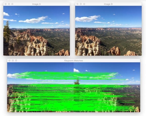
At the top of this figure, we can see two input images (resized to fit on my screen, the raw .jpg files are a much higher resolution). And on the bottom, we can see the matched keypoints between the two images.

Using these matched keypoints, we can apply a perspective transform and obtain the final panorama:

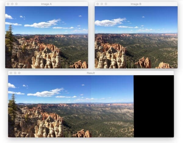
As we can see, the two images have been successfully stitched together!

Note: On many of these example images, you’ll often see a visible “seam” running through the center of the stitched images. This is because I shot many of photos using either my iPhone or a digital camera with autofocus turned on, thus the focus is slightly different between each shot. Image stitching and panorama construction work best when you use the same focus for every photo. I never intended to use these vacation photos for image stitching, otherwise I would have taken care to adjust the camera sensors. In either case, just keep in mind the seam is due to varying sensor properties at the time I took the photo and was not intentional.

Let’s give another set of images a try:

$ python stitch.py --first images/bryce_left_02.png \
	--second images/bryce_right_02.png

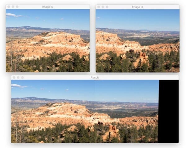
Again, our Stitcher class was able to construct a panorama from the two input images.

Now, let’s move on to the Grand Canyon:

$ python stitch.py --first images/grand_canyon_left_01.png \
	--second images/grand_canyon_right_01.png

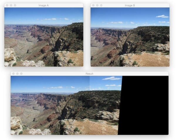
In the above input images we can see heavy overlap between the two input images. The main addition to the panorama is towards the right side of the stitched images where we can see more of the “ledge” is added to the output.

Here’s another example from the Grand Canyon:

$ python stitch.py --first images/grand_canyon_left_02.png \
	--second images/grand_canyon_right_02.png

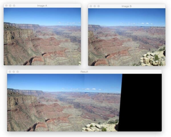
From this example, we can see that more of the huge expanse of the Grand Canyon has been added to the panorama.

Finally, let’s wrap up this blog post with an example image stitching from Sedona, AZ:

$ python stitch.py --first images/sedona_left_01.png \
	--second images/sedona_right_01.png

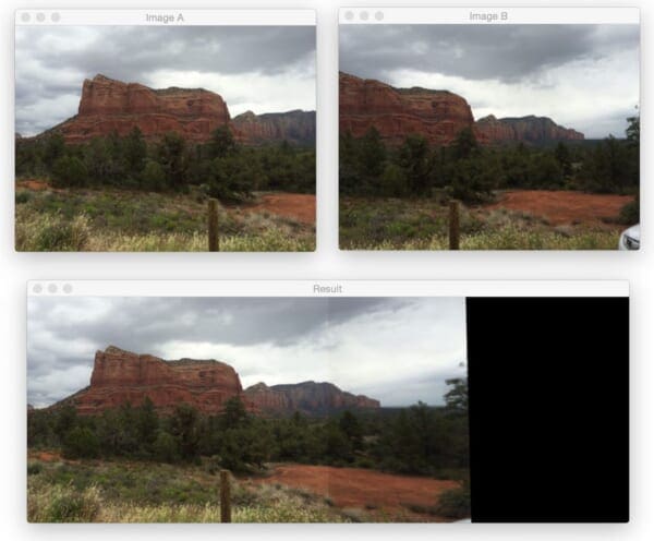
Personally, I find the red rock country of Sedona to be one of the most beautiful areas I’ve ever visited. If you ever have a chance, definitely stop by — you won’t be disappointed.

So there you have it, image stitching and panorama construction using Python and OpenCV!

Summary

In this blog post we learned how to perform image stitching and panorama construction using OpenCV. Source code was provided for image stitching for both OpenCV 2.4 and OpenCV 3.

Our image stitching algorithm requires four steps: (1) detecting keypoints and extracting local invariant descriptors; (2) matching descriptors between images; (3) applying RANSAC to estimate the homography matrix; and (4) applying a warping transformation using the homography matrix.

While simple, this algorithm works well in practice when constructing panoramas for two images. In a future blog post, we’ll review how to construct panoramas and perform image stitching for more than two images.

Anyway, I hope you enjoyed this post! Be sure to use the form below to download the source code and give it a try.