Training a Custom Image Classification Network for OAK-D

---

Table of Contents

---

Training a Custom Image Classification Network for OAK-D

In this tutorial, you will learn to train a custom image classification network for OAK-D using the TensorFlow framework. Furthermore, this tutorial aims to develop an image classification model that can learn to classify one of the 15 vegetables (e.g., tomato, brinjal, and bottle gourd).

If you are a regular PyImageSearch reader and have even basic knowledge of Deep Learning in Computer Vision, then this tutorial should be easy to understand. Furthermore, this tutorial acts as a foundation for the following tutorial, where we learn to deploy this trained image classification model on OAK-D.

This is the 3rd lesson in our 4-part series on OAK 101:

1. Introduction to OpenCV AI Kit (OAK)
2. OAK-D: Understanding and Running Neural Network Inference with DepthAI API
3. Training a Custom Image Classification Network for OAK-D (today’s tutorial)
4. Deploying a Custom Image Classifier on an OAK-D

To learn how to train an image classification network for OAK-D, just keep reading.

---

Training a Custom Image Classification Network for OAK-D

Before we start data loading, analysis, and training the classification network on the data, we must carefully pick the suitable classification architecture as it would finally be deployed on the OAK. Although OAK can process 4 trillion operations per second, it is still an edge device. It has its bottlenecks, so we cannot expect it to run a heavyweight model like EfficientNet-B7, achieving real-time inference speed.

In today’s experiment, we would use MobileNetV2 as a feature extractor pre-trained on ImageNet data. MobileNetV2 is a classification model developed by Google. It provides real-time classification capabilities under computing constraints in edge devices. Hence, the obvious choice for this tutorial.

We would add custom layers on top of the MobileNetV2 pre-trained feature extractor, and these layers would be trained to perform image classification while the feature extractor (base model) weights would be frozen (non-trainable).

In short, we would perform Transfer learning that takes features learned on one problem and leverage them on a new, similar problem. For example, features from the base model that has learned to identify 1000-ImageNet classes would be helpful to give a head start to a model meant to identify vegetables.

---

Configuring Your Development Environment

To follow this guide, you need to have tensorflow, scikit-learn, and matplotlib installed on your system.

Luckily, all these libraries are pip-installable:

$ pip install tensorflow==2.9.2
$ pip install scikit-learn==0.23.2
$ pip install matplotlib==3.3.2

---

Having Problems Configuring Your Development Environment?

All that said, are you:

• Short on time?
• Learning on your employer’s administratively locked system?
• Wanting to skip the hassle of fighting with the command line, package managers, and virtual environments?
• Ready to run the code right now on your Windows, macOS, or Linux system?

Then join PyImageSearch University today!

Gain access to Jupyter Notebooks for this tutorial and other PyImageSearch guides that are pre-configured to run on Google Colab’s ecosystem right in your web browser! No installation required.

And best of all, these Jupyter Notebooks will run on Windows, macOS, and Linux!

---

Project Structure

We first need to review our project directory structure.

Start by accessing the “Downloads” section of this tutorial to retrieve the source code and example images.

From there, take a look at the directory structure:

├── output
│   ├── accuracy_loss_plot.png
│   ├── test_prediction_images.png
│   └── vegetable_classifier
│       ├── keras_metadata.pb
│       ├── saved_model.pb
│       └── variables
│           ├── variables.data-00000-of-00001
│           └── variables.index
├── pyimagesearch
│   ├── __init__.py
│   ├── config.py
│   ├── network.py
│   └── utils.py
├── test.py
└── train.py

In the pyimagesearch directory, we have the following:

• config.py: The configuration file for the experiments
• utils.py: The utilities for the image classification training
• network.py: Houses the implementation of the end-to-end classification model (i.e., the base MobileNetV2 model) and the classification layers

In the core directory, we have 3 files:

• requirements.txt: The Python packages that are required for this tutorial
• train.py: It contains the script for training the image classification model
• test.py: Script that runs an inference of the trained classification model on test data

---

The Vegetable Image Dataset

Before we go ahead and load the data, it’s good to look at what you’ll exactly be working with! The Vegetable Image Dataset comprises 15 vegetable images, with 224×224 color images of 21,000 different vegetables from 15 categories and 1400 images per category. The training set has 15,000 images, and the validation and test sets have 3,000 images each. You can double-check this later when you have loaded your data!

The good news is that the image dimensions are already what our pretrained MobileNetV2 model expects (i.e., 224×224), so we do not need to worry about resizing, but we still do that as a sanity check step.

Before you load this data, you need to download it from Kaggle. We show how to download this dataset in our Google Colab in very few steps, so check that out!

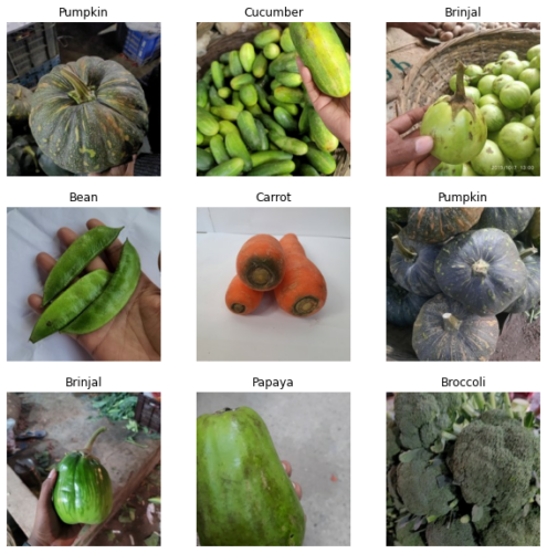
Figure 2 shows 9 of the 15 vegetable image categories from the dataset. At first glance, the dataset has a good amount of variation within the image. For example, brinjal is present at multiple scales in the image. But we would still apply data augmentation to ensure the model doesn’t overfit and generalize well on the test dataset.

---

Data Analysis

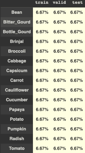
When working with data, especially supervised learning, it is often a best practice to check data imbalance. For example, Figure 3 shows the percentage of each vegetable (category) across different splits (train, valid, and test), and it clearly shows that the data is perfectly balanced across all splits.

---

Configuring the Prerequisites

Before we start our implementation, let’s go over the configuration pipeline of our project. We will move on to the config.py script located in the pyimagesearch directory.

# import the necessary packages
import os

# define the base path, paths to separate train, validation, and test splits
BASE_DATASET_PATH = "datasets/Vegetable Images"
TRAIN_DATA_PATH = os.path.join(BASE_DATASET_PATH, "train")
VALID_DATA_PATH = os.path.join(BASE_DATASET_PATH, "validation")
TEST_DATA_PATH = os.path.join(BASE_DATASET_PATH, "test")
OUTPUT_PATH = "output"

# define the image size and the batch size of the dataset
IMAGE_SIZE = 224
BATCH_SIZE = 32

# number of channels, 1 for gray scale and 3 for color images
CHANNELS = 3

# define the classifier network learning rate
LR_INIT = 0.0001

# number of epochs for training
NUM_EPOCHS = 20

# number of categories/classes in the dataset
N_CLASSES = 15

# define paths to store training plots, testing prediction and trained model
ACCURACY_LOSS_PLOT_PATH = os.path.join("output", "accuracy_loss_plot.png")
TRAINED_MODEL_PATH = os.path.join("output", "vegetable_classifier")
TEST_PREDICTION_OUTPUT = os.path.join("output", "test_prediction_images.png")

The config.py helps set up the file paths and parameters for the dataset and the classifier network that will train and test the image classification model.

We start by importing the os package to help us create datasets and output paths. Then, from Lines 5-9, we set the base path for the dataset and define the paths for the train, validation, and test splits of the dataset and the output path.

On Lines 12 and 13, we define the dataset’s image and batch sizes. Then determine the number of channels set to 3 for color images, the classifier network learning rate, the number of epochs for training, and the number of categories/classes in the dataset (Lines 16-25).

Finally, on Lines 28-30, we define the paths to store the training plots, testing predictions, and the trained model.

---

Defining the Utilities

Now that the configuration pipeline has been defined, we can define the training utilities. The utils.py script defines several functions:

• prepare the dataset for training
• apply data augmentation and normalization of the input images
• define early stopping callbacks to stop the training if the validation loss does not improve

We will use these functions in the training process to make the model more robust.

from pyimagesearch import config
import tensorflow as tf

def prepare_batch_dataset(data_path, img_size, batch_size, shuffle=True):
	return tf.keras.preprocessing.image_dataset_from_directory(
		data_path,
		image_size=(img_size, img_size),
		shuffle=shuffle,
		batch_size=batch_size
	)

On Lines 1 and 2, we import config from the pyimagesearch module and the TensorFlow library.

From Lines 4-10, we define the function prepare_batch_dataset that takes in the following:

• path of the dataset
• image size
• batch size
• boolean value for shuffle

It then uses tf.keras.preprocessing.image_dataset_from_directory to load the images from the directory, resizes them to the given image size, shuffles them if shuffle is True, and returns the dataset in the form of batches.

def callbacks():
	# build an early stopping callback and return it
	callbacks = [
		tf.keras.callbacks.EarlyStopping(
			monitor="val_loss",
			min_delta=0,
			patience=2,
			mode="auto",
		),
	]
	return callbacks

On Lines 12-22, the function callbacks defines an early stopping callback and returns it. The callback monitors the validation loss and stops the training if it does not improve after two epochs.

def normalize_layer(factor=1./127.5):
	# return a normalization layer
	return tf.keras.layers.Rescaling(factor, offset=-1)

def augmentation():
	# build a sequential model with augmentations
	data_aug = tf.keras.Sequential(
		[
			tf.keras.layers.RandomFlip("horizontal"),
			tf.keras.layers.RandomRotation(0.1),
			tf.keras.layers.RandomZoom(0.1),
		]
	)
	return data_aug

Then on Lines 24-26, the function normalize_layer returns a normalization layer. It normalizes the input data by dividing by 127.5 and subtracting 1. In short, it normalizes or scales the input images from [0, 255] to [-1, 1], which is what the MobileNetV2 network expects.

Finally, from Lines 28-37, the function augmentation creates a sequential model with image augmentations: random horizontal flipping, rotation, and zoom. The augmentation helps avoid overfitting and allows the model to generalize better.

---

The Image Classification Network

Now with the utilities defined, we head towards coding the most exciting part (i.e., the image classification network). If you haven’t coded an image classification network before, the section is definitely for you! So let’s get straight into the code.

# import the necessary packages
from pyimagesearch.utils import augmentation
from pyimagesearch.utils import normalize_layer
import tensorflow as tf

class MobileNet:
	@staticmethod
	def build(width, height, depth, classes):
		# initialize the pretrained mobilenet feature extractor model
		# and set the base model layers to non-trainable
		base_model = tf.keras.applications.MobileNetV2(
			input_shape=(height, width, depth),
			include_top=False,
			weights="imagenet",
		)

We start by importing the necessary packages on Lines 2-4, including the augmentation and normalize_layer modules from the pyimagesearch library and TensorFlow as tf.

On Line 6, a class called MobileNet is defined. Within this class, a static method called build takes four arguments: width, height, depth, and classes.

From Lines 11-15, we define the base_model variable, which is the MobileNetV2 architecture with the input shape set to (height, width, depth), include_top set to False, and weights set to imagenet.

		base_model.trainable = False

Then, on Line 16, the base model’s trainable attribute is set to False so that the model’s base layers are not trainable.

		# define the input to the classification network with
		# image dimensions
		inputs = tf.keras.Input(shape=(height, width, depth))

On Line 20, the input to the model is defined as a tensor with shape (height, width, depth) and named inputs.

		# apply augmentation to the inputs and normalize the batch
		# images to [-1, 1] as expected by MobileNet
		x = augmentation()(inputs)
		x = normalize_layer()(x)

Then on Lines 24 and 25, an augmentation layer is applied to the inputs, and the normalized layer is applied to the augmented inputs, which scales the input pixels to [-1, 1].

		# pass the normalized and augmented images to base model,
		# average the 7x7x1280 into a 1280 vector per image,
		# add dropout as a regularizer with dropout rate of 0.2
		x = base_model(x, training=False)
		x = tf.keras.layers.GlobalAveragePooling2D()(x)
		x = tf.keras.layers.Dropout(0.2)(x)

The normalized and augmented inputs are then passed through the base model on Line 30. Next, the output of the base model is passed through a global average pooling layer (on Line 31). Then, on Line 32, a dropout layer is applied with a dropout rate of 0.2.

		# apply dense layer to convert the feature vector into
		# a prediction of classes per image
		outputs = tf.keras.layers.Dense(classes)(x)

		# build the keras Model by passing input and output of the
		# model and return the model
		model = tf.keras.Model(inputs, outputs)
		return model

On Line 36, a dense layer with classes as the number of outputs is applied to the dropout layer’s output. This dense layer will convert the feature vector into predictions of classes per image.

Finally, on Lines 40 and 41, a Keras Model is built by passing the inputs and outputs to the Model class, and the model is returned to the calling function.

---

Training

With the configurations, helper functions, and, notably, the image classification network implemented, we can finally get into the code walkthrough of training the classification neural network.

# USAGE
# python train.py

# import the necessary packages
from pyimagesearch.utils import prepare_batch_dataset
from pyimagesearch.utils import callbacks
from pyimagesearch import config
from pyimagesearch.network import MobileNet
from matplotlib import pyplot as plt
import tensorflow as tf
import os

# build the training and validation dataset pipeline
print("[INFO] building the training and validation dataset...")
train_ds = prepare_batch_dataset(
	config.TRAIN_DATA_PATH, config.IMAGE_SIZE, config.BATCH_SIZE
)

val_ds = prepare_batch_dataset(
	config.VALID_DATA_PATH, config.IMAGE_SIZE, config.BATCH_SIZE
)

The script starts by importing necessary packages such as the prepare_batch_dataset, callbacks, config, MobileNet, and pyplot from matplotlib. The script also imports TensorFlow as tf and os (Lines 5-11).

On Lines 15-21, a pipeline for the training and validation datasets is built. The function prepare_batch_dataset is used to create the dataset by passing in the path of the training data, image size, and batch size, as specified in the config file. The same is done for the validation dataset.

# build the output path if not already exists
if not os.path.exists(config.OUTPUT_PATH):
	os.makedirs(config.OUTPUT_PATH)

# initialize the callbacks, model, optimizer and loss
print("[INFO] compiling model...")
callbacks = callbacks()
model = MobileNet.build(
	width=config.IMAGE_SIZE,
	height=config.IMAGE_SIZE,
	depth=config.CHANNELS,
	classes=config.N_CLASSES
)
optimizer = tf.keras.optimizers.Adam(learning_rate=config.LR_INIT)
loss = tf.keras.losses.SparseCategoricalCrossentropy(from_logits=True)

# compile the model
model.compile(
	optimizer=optimizer,
	loss=loss,
	metrics=["accuracy"]
)

Then, on Lines 24 and 25, the output path is created if it doesn’t already exist.

From Lines 29-44,

• The model is compiled by initializing the callbacks, model, optimizer, and loss.
• The model is built by calling the build method of the MobileNet class and passing in the width, height, depth, and number of classes as specified in the config file.
• The Adam optimizer is used with the initial learning rate specified in the config file, and the loss function used is sparse categorical cross-entropy.

# evaluate the model initially
(initial_loss, initial_accuracy) = model.evaluate(val_ds)
print("initial loss: {:.2f}".format(initial_loss))
print("initial accuracy: {:.2f}".format(initial_accuracy))

# train the image classification network
print("[INFO] training network...")
history = model.fit(
	train_ds,
	epochs=config.NUM_EPOCHS,
	validation_data=val_ds,
	callbacks=callbacks,
)

The initial loss and accuracy of the model are evaluated on the validation dataset on Line 47.

From Lines 53-58, the model is trained by calling the fit method on the model with the training dataset and passing in the number of epochs specified in the config file and the validation dataset. The callbacks are passed in as well during training.

# save the model to disk
print("[INFO] serializing network...")
model.save(config.TRAINED_MODEL_PATH)

# save the training loss and accuracy plot
plt.style.use("ggplot")
acc = history.history['accuracy']
val_acc = history.history['val_accuracy']

loss = history.history['loss']
val_loss = history.history['val_loss']

plt.figure(figsize=(8, 8))
plt.subplot(2, 1, 1)
plt.plot(acc, label='Training Accuracy')
plt.plot(val_acc, label='Validation Accuracy')
plt.legend(loc='lower right')
plt.ylabel('Accuracy')
plt.ylim([min(plt.ylim()),1])
plt.title('Training and Validation Accuracy')

plt.subplot(2, 1, 2)
plt.plot(loss, label='Training Loss')
plt.plot(val_loss, label='Validation Loss')
plt.legend(loc='upper right')
plt.ylabel('Cross Entropy')
plt.ylim([0,1.0])
plt.title('Training and Validation Loss')
plt.xlabel('epoch')
plt.savefig(config.ACCURACY_LOSS_PLOT_PATH)

We save the model to the disk on Line 62 using the save method and the path specified in the config file.

Finally, from Lines 65-89, the training loss and accuracy are plotted using matplotlib and saved to a file using the path specified in the config file.

---

Accuracy and Loss Plots: Training vs. Validation

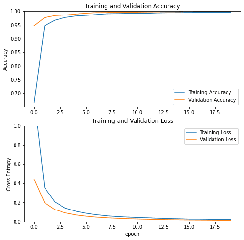
From Figure 4, you can see that the validation loss and validation accuracy are almost in sync with the training loss and training accuracy. It’s a good validation that the model is balanced: the validation loss is decreasing and not increasing, and there is not much gap between training and validation accuracy. In fact, after 10 epochs, the training and validation curves coincide.

Therefore, your model’s generalization capability is good, but the test set could be challenging, and the model might not perform well.

---

Testing

Finally, it’s time to put our trained model to the test and see how well it performs on the test set. In this last section of the tutorial, we will run inference on the test data and plot the classification report and a few test images with their respective predicted class labels.

# USAGE
# python test.py

# import the necessary packages
from pyimagesearch.utils import prepare_batch_dataset
from pyimagesearch.utils import callbacks
from pyimagesearch import config
from pyimagesearch.network import MobileNet
from sklearn.metrics import classification_report
from matplotlib import pyplot as plt
import tensorflow as tf
import numpy as np
import os

# build the test dataset pipeline with and without shuffling the dataset
print("[INFO] building the test dataset with and without shuffle...")
test_ds_wo_shuffle = prepare_batch_dataset(
	config.TEST_DATA_PATH,
	config.IMAGE_SIZE,
	config.BATCH_SIZE,
	shuffle=False
)

test_ds_shuffle = prepare_batch_dataset(
	config.TEST_DATA_PATH, config.IMAGE_SIZE, config.BATCH_SIZE
)

We start by importing necessary packages such as the prepare_batch_dataset, callbacks, config, MobileNet, classification_report from sklearn, pyplot from matplotlib, numpy, and tensorflow on Lines 5-13.

Then on Lines 17-26, the test datasets are created with and without shuffling, using the prepare_batch_dataset function with the path of the test data, image size, and batch size, as specified in the config file.

We created without shuffling to have an association between the test data ground-truth labels and predicted labels for computing the classification report.

# load the trained image classification convolutional neural network
model = tf.keras.models.load_model(config.TRAINED_MODEL_PATH)
# print model summary on the terminal
print(model.summary())

# evaluate the model on test dataset and print the test accuracy
loss, accuracy = model.evaluate(test_ds_wo_shuffle)
print("Test accuracy :", accuracy)

# fetch class names
class_names = test_ds_wo_shuffle.class_names

# generate classification report by (i) predicting on test dataset
# (ii) take softmax of predictions (iii) for each sample in test set
# fetch index with max. probability (iv) create a vector of true labels
# (v) pass ground truth, prediction for test data along with class names
# to classification_report method
test_pred = model.predict(test_ds_wo_shuffle)
test_pred = tf.nn.softmax(test_pred)
test_pred = tf.argmax(test_pred, axis=1)
test_true_labels = tf.concat(
	[label for _, label in test_ds_wo_shuffle], axis=0
)
print(
	classification_report(
		test_true_labels, test_pred, target_names=class_names
	)
)

On Lines 29-31, the pre-trained model is loaded from the path specified in the config file. Its summary is printed on the terminal.

Then on Lines 34 and 35, the model is evaluated on the test dataset (without shuffling). The accuracy is printed on the terminal.

On Lines 45-55, a classification report is generated by

• predicting on the test dataset
• applying softmax to the predictions
• fetching the index with the maximum probability for each sample in the test set
• creating a vector of true labels
• passing that, along with the class names, to the classification_report method from sklearn

# Retrieve a batch of images from the test set and run inference
image_batch, label_batch = test_ds_shuffle.as_numpy_iterator().next()
predictions = model.predict_on_batch(image_batch)

# Apply a softmax
score = tf.nn.softmax(predictions)
print(score.shape)

# save the plot for model prediction along with respective test images
plt.figure(figsize=(10, 10))
for i in range(9):
	ax = plt.subplot(3, 3, i + 1)
	plt.imshow(image_batch[i].astype("uint8"))
	plt.title(class_names[np.argmax(score[i])])
	plt.axis("off")
plt.savefig(config.TEST_PREDICTION_OUTPUT)

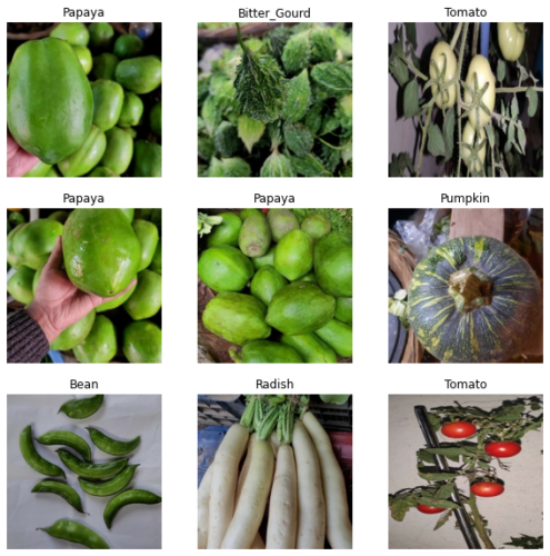
On Lines 58-62, we retrieve a batch of images from the test set, run inference on it, and apply softmax.

Finally, from Lines 66-72, a plot is created of the model’s predictions along with their respective images from the test set, and it is saved to the path specified in the config file.

---

Classification Report

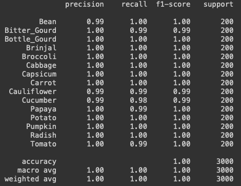
Figure 5 summarizes how the model performs on each of the 15 classes with help from the precision and recall metrics. Figure 5 also shows that the model does exceptionally well in all the classes.

Apart from the categories: Bean, Bitter_Gourd, Cauliflower, Cucumber, Papaya, and Tomato, all other classes have 100% f1-score (harmonic average of precision and recall). This is an excellent validation for the model we trained on the vegetable classification dataset.

---

Sample Test Set Predictions

We have already seen the quantitative results in detail for each class through a classification report; in Figure 6, we show few qualitative results, the predictions made by the trained image classification model on the test set.

---

Summary

In this tutorial, we trained an image classification neural network on a vegetable image classification dataset from Kaggle.

The image classification network consisted of MobileNetV2 as the base model for feature extraction pre-trained on the ImageNet dataset. The classification layers were added to the base model to convert the feature vectors into class predictions.

The model performed exceptionally well on the test dataset provided on Kaggle. Based on the classification report, the model achieved almost 100% accuracy across all classes.

As we mentioned earlier, this tutorial was an essential foundation for our following tutorial in the OAK-101 course, where we will learn to deploy this image classification model. In addition, we will learn to convert the TensorFlow framework model to the format OAK expects.

Also, we will learn to use DepthAI API to run inference on OAK with images and camera video streams.

---

Citation Information

Sharma, A. “Training a Custom Image Classification Network for OAK-D,” PyImageSearch, P. Chugh, A. R. Gosthipaty, S. Huot, K. Kidriavsteva, R. Raha, and A. Thanki, eds., 2023, https://pyimg.co/ab1dj

@incollection{Sharma_2023_CIC-OAK-D,
  author = {Aditya Sharma},
  title = {Training a Custom Image Classification Network for {OAK-D}},
  booktitle = {PyImageSearch},
  editor = {Puneet Chugh and Aritra Roy Gosthipaty and Susan Huot and Kseniia Kidriavsteva and Ritwik Raha and Abhishek Thanki},
  year = {2023},
  url = {https://pyimg.co/ab1dj},
}

---

---

To download the source code to this post (and be notified when future tutorials are published here on PyImageSearch), simply enter your email address in the form below!