A Brief Introduction to Do-Calculus

Welcome back to Part 4 of the series on Causality in Machine Learning. The previous two parts introduced us to the world of causal inference and the various methodologies involved.

In this part, we will discuss a very popular and useful method known as the do-calculus developed by Judea Pearl in 1995. It was developed to propose a foolproof methodology for the identification of causal effects in non-parametric models.

Well, that’s a mouthful. What do we mean by that?

In simple words, this means to identify the effect or effects for a particular cause from data that is continuous rather than having discrete values.

We have learned in the previous blogs that it is impossible to do Causal Inference without having some form of intervention on the provided data. To facilitate this, do-calculus introduces a mathematical operator called $\text{do}(x)$ , which simulates intervention by removing certain functions from the model and replacing them with a constant $X=x$ . To understand how this plays out, we will first have to look at some of the definitions introduced by Pearl.

Definitions

Definition 1

The probability distribution of the outcome $Y$ after the intervention is given by the equation:

$P_M(y \mid \text{do}(x)) = P_{M_x}(y)$

where the distribution of the outcome $Y$ is defined as the probability assigned by the model $M_x$ to each outcome level $Y=y$ .

Definition 2

This part discusses when and under what conditions a causal query (whether a variable or a group of variables is the cause for a given effect or not) is identifiable.

Given a set of assumptions ( $A$ ) that satisfy two fully specified models ( $M_1$ and $M_2$ ), the following is the criteria for identifiability:

$P(M_1) = P(M_2) \Rightarrow Q(M_1) = Q(M_2)$

This means that whatever the details of the models are, if the distribution of the two models given the same set of assumptions ( $A$ ) are equal, then it follows that the causal query for the two models should also be equal. This can be extended to mean that a causal query, under such circumstances, can be expressed in terms of the parameters of $P$ .

The Rules of Do-Calculus

Now that we have learned about the definitions of do-calculus, let us familiarize ourselves with the three rules that govern the mathematics of do-calculus. But first, we need to understand the necessity of these rules.

In the previous section, we learned under what conditions a causal query will be identifiable, and we also saw how to formulate an expression in terms of a do-expression (e.g., $P_M(y \mid \text{do}(x)) = P_{M_x}(y)$ ). So, when a causal query is given to us in the form of a do-expression, there are actual mathematical steps that can be taken to resolve it and find out whether the query is identifiable or not.

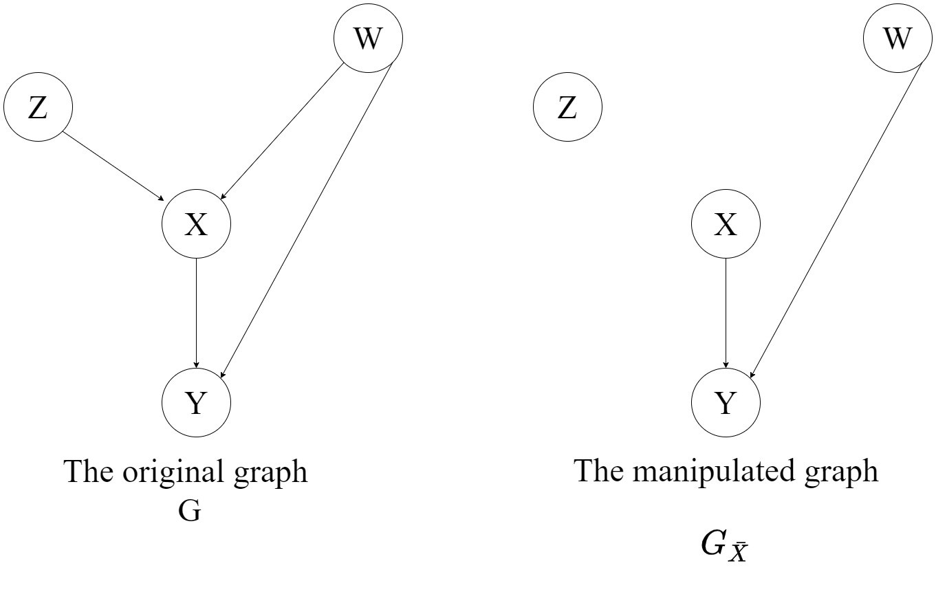
Consider the following directed acyclic graph in Figure 1 ( $G$ ) where $X$ , $Y$ , $Z$ , and $W$ are arbitrary disjoint nodes. $G{}_{\overline{X}}$ is the manipulated graph where all incoming edges to $X$ have been removed.

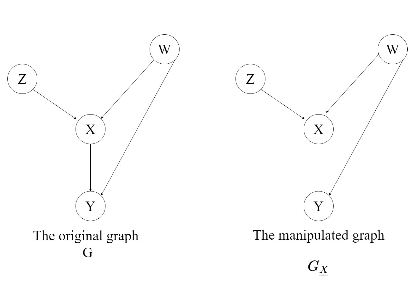
**Figure 1:** Original and manipulated graphs (source: image by the authors).

Similarly, $G_{\underline{X}}$ is the manipulated graph where all outgoing edges to $X$ have been removed, as shown in Figure 2.

**Figure 2:** Outgoing graphs (source: image by the authors).

Another useful notation to get familiarized with is the concept of $d$ -separation ( $\perp\!\!\!\perp$ ). In very simple words, given the graph, $a \rightarrow c \rightarrow b$ , the expression $a \perp\!\!\!\perp b \mid c$ means that $a$ is conditionally independent of $b$ given $c$ .

To understand $d$ -separation in a more detailed manner, have a look at this single-page explanation.

Rule 1: Insertion/Deletion of Observation

$P(y \mid \text{do}(x),z,w) = P(y \mid \text{do}(x),w)$ if $(Y \perp\!\!\!\perp Z \mid X,W)$ for $G{}_{\overline{X}}$ .

This means that if $Y$ is $d$ -separated from $Z$ given $X$ and $W$ , then the expression of probability $P(y \mid \text{do}(x),z,w)$ resolves to $P(y \mid \text{do}(x),w)$ . An easier way to understand this is by getting rid of the do-operators on both sides of the equality sign.

$P(y \mid z,w) = P(y \mid w)$ if $(Y \perp\!\!\!\perp Z \mid W)$ for $G$

The above expression simply implies conditional independence within the variables in the distribution given regular $d$ -separation.

Rule 2: Action/Observation Exchange

$P(y \mid \text{do}(x),\text{do}(z),w) = P(y \mid \text{do}(x),z,w)$ if $(Y \perp\!\!\!\perp Z \mid X,W)$ for $G{}_{\overline{X}\underline{Z}}$ .

To simplify the expression above, let us again remove $\text{do}(x)$ or consider $X$ to be an empty set.

$P(y \mid \text{do}(z),w) = P(y \mid z,w)$ if $(Y \perp\!\!\!\perp Z \mid W)$ for $G_{\underline{Z}}$ .

This expression refers to the backdoor-adjustment criteria that we saw in Part 3. Therefore, this rule gives us the interventional distribution for the backdoor adjustment criteria.

Rule 3: Insertion/Deletion of Action

$P(y \mid \text{do}(x), \text{do}(z),w) = P(y \mid \text{do}(x),w)$ if $(Y \perp\!\!\!\perp Z \mid X,W)$ for $G{}_{\overline{X}\, \overline{Z(W)}}$

where $Z(W)$ is the set of $Z$ nodes that are not ancestors of any $W$ node in $G{}_{\overline{X}}$ .

Again, for the sake of simplification, let us remove the $\text{do}(x)$ operator from the above expression.

$P(y \mid \text{do}(z),w) = P(y \mid w)$ if $(Y \perp\!\!\!\perp Z \mid W)$ for $G{}_{\overline{Z(W)}}$

Let’s pause here and really understand what this means. On the paper, it means that we can remove the intervention term $\text{do}(z)$ provided there is no causal association flowing from $Z$ to $Y$ $(Y \perp\!\!\!\perp Z \mid W)$ in the graph $G{}_{\overline{Z(W)}}$ .

But that’s not all. We have a strange term called $Z(W)$ , which doesn’t quite fit in.

The simplified expression should have been:

$P(y \mid \text{do}(z),w) = P(y \mid w)$ if $(Y \perp\!\!\!\perp Z \mid W)$ for $G{}_{\overline{Z}}$

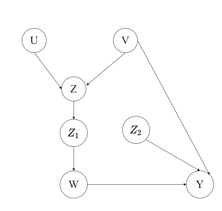
where removal of incoming edges to $Z$ should result in the $d$ -separation of $Y$ and $Z$ , and no causal association should flow from $Z$ to $Y$ . However, instead of this simple term, we end up with an expression containing $Z(W)$ . To understand this better, let us consider Figure 3:

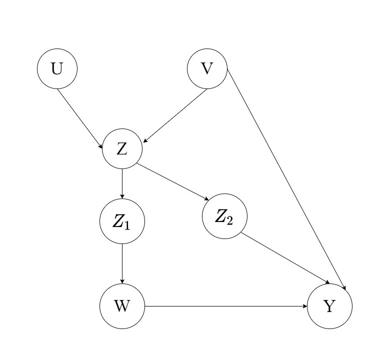**Figure 3:** $d$ -separation (source: image by the authors).

Now, the intuitive idea is to remove incoming edges to $Z$ ( $G{}_{\overline{Z}}$ ). But if we do that, then we risk changing the distribution of $Y$ altogether through the backdoor path consisting of $U$ and $V$ .

Instead, what we can do is take a sub-node of $Z$ , say $Z_2$ , which is not an ancestor of any node in $W$ , and then remove all the incoming edges to it ( $G{}_{\overline{Z_2}}$ ). This is shown in Figure 4.

**Figure 4:** Removing incoming edges (source: image by the authors).

What's next? We recommend PyImageSearch University.

Course information:
86+ total classes • 115+ hours hours of on-demand code walkthrough videos • Last updated: May 2025
★★★★★ 4.84 (128 Ratings) • 16,000+ Students Enrolled

I strongly believe that if you had the right teacher you could master computer vision and deep learning.

Do you think learning computer vision and deep learning has to be time-consuming, overwhelming, and complicated? Or has to involve complex mathematics and equations? Or requires a degree in computer science?

That’s not the case.

All you need to master computer vision and deep learning is for someone to explain things to you in simple, intuitive terms. And that’s exactly what I do. My mission is to change education and how complex Artificial Intelligence topics are taught.

If you're serious about learning computer vision, your next stop should be PyImageSearch University, the most comprehensive computer vision, deep learning, and OpenCV course online today. Here you’ll learn how to successfully and confidently apply computer vision to your work, research, and projects. Join me in computer vision mastery.

Inside PyImageSearch University you'll find:

✓ 86+ courses on essential computer vision, deep learning, and OpenCV topics
✓ 86 Certificates of Completion
✓ 115+ hours hours of on-demand video
✓ Brand new courses released regularly, ensuring you can keep up with state-of-the-art techniques
✓ Pre-configured Jupyter Notebooks in Google Colab
✓ Run all code examples in your web browser — works on Windows, macOS, and Linux (no dev environment configuration required!)
✓ Access to centralized code repos for all 540+ tutorials on PyImageSearch
✓ Easy one-click downloads for code, datasets, pre-trained models, etc.
✓ Access on mobile, laptop, desktop, etc.

Click here to join PyImageSearch University

Summary

The rules and definitions of do-calculus provide a general structure for identifying Causal queries. The final query $Q$ should be free of any do-operator. This can be achieved by repeatedly applying the three rules. It is also complete, meaning if there exists a Causal Query $Q$ that is identifiable, then it can be identified using do-calculus.

This lesson was aimed at introducing do-calculus very briefly and laying down the rules of the game. The idea is not to intimidate any newcomer with a whole lot of mathematical jargon but to provide insight into an essentially simple yet powerful framework for causal inference.

References

Citation Information

A. R. Gosthipaty and R. Raha. “A Brief Introduction to Do-Calculus,” PyImageSearch, P. Chugh, S. Huot, and K. Kidriavsteva, eds., 2023, https://pyimg.co/h3q2n

@incollection{ARG-RR_2023_IntroDoCalculus,
  author = {Aritra Roy Gosthipaty and Ritwik Raha},
  title = {A Brief Introduction to Do-Calculus},
  booktitle = {PyImageSearch},
  editor = {Puneet Chugh and Susan Huot and Kseniia Kidriavsteva},
  year = {2023},
  url = {https://pyimg.co/h3q2n},
}

Unleash the potential of computer vision with Roboflow - Free!

Step into the realm of the future by signing up or logging into your Roboflow account. Unlock a wealth of innovative dataset libraries and revolutionize your computer vision operations.
Jumpstart your journey by choosing from our broad array of datasets, or benefit from PyimageSearch’s comprehensive library, crafted to cater to a wide range of requirements.
Transfer your data to Roboflow in any of the 40+ compatible formats. Leverage cutting-edge model architectures for training, and deploy seamlessly across diverse platforms, including API, NVIDIA, browser, iOS, and beyond. Integrate our platform effortlessly with your applications or your favorite third-party tools.
Equip yourself with the ability to train a potent computer vision model in a mere afternoon. With a few images, you can import data from any source via API, annotate images using our superior cloud-hosted tool, kickstart model training with a single click, and deploy the model via a hosted API endpoint. Tailor your process by opting for a code-centric approach, leveraging our intuitive, cloud-based UI, or combining both to fit your unique needs.
Embark on your journey today with absolutely no credit card required. Step into the future with Roboflow.

Join Roboflow Now

Join the PyImageSearch Newsletter and Grab My FREE 17-page Resource Guide PDF

Enter your email address below to join the PyImageSearch Newsletter and download my FREE 17-page Resource Guide PDF on Computer Vision, OpenCV, and Deep Learning.

Table of Contents