Spatial Transformer Networks Using TensorFlow

---

Table of Contents

---

Convolution Neural Networks (CNNs) have undoubtedly altered the way the technology world operates. Having established itself in the world of image processing, the number of subdomains it has impacted are too many to count.

It is as if we have solved the problem of teaching a computer about images with just mere matrix multiplications and some calculus. However, it’s not as perfect as it seems.

Let us see what I mean by this. In Figure 1, we have a standard CNN numerical digit predictor.

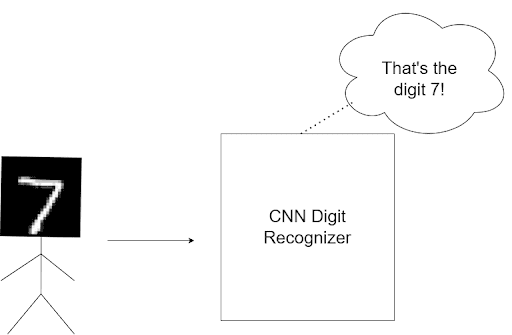
With enough data, it’ll work exactly how it’s expected to, showcasing the power of CNNs. However, what happens when you rotate the figure and feed it to the model (Figure 2)?

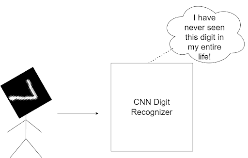
Despite their ingenious nature, CNNs are not transformation invariant. This means if I so much as rotate the image, the CNN will, in all likelihood, predict the wrong answer, leading us to conclude that CNNs are NOT transformally invariant.

Now you might think that this isn’t a huge issue. However, this is where the uncertainty factor of the real world comes in.

Let’s take the example of a number plate detector. Even if it estimates the general area of the number plate, it might mislabel the digits if the detected region is not horizontal. Imagine how much inconvenience this might cause in a busy toll plaza commute.

The intuition behind this is very interesting. Our eyes can detect the number 7 no matter how much you twist the input image. A big reason is that we only care about the digit, not the background while processing the image in our brains.

For a machine learning model, the complete pixel orientation is considered, not just the digit. After all, machine learning models are matrices. Therefore, the values of these weight matrices are formed depending on the complete pixel orientations of the input data.

So for a concept this brilliant, isn’t this a big bummer?

Thankfully, the ever-fast researchers of the deep learning world have already come up with a solution, that is, Spatial Transformer Networks.

To learn how to implement Spatial Transformer Networks, just keep reading.

---

Spatial Transformer Networks Using TensorFlow

The main intention behind the Spatial Transformer network module is to help our model choose the most relevant ROI of images. Once the model successfully figures out the relevant pixels, the spatial transformation module will help the model decide what kind of transformation is necessary for the image to become standard format.

Remember, the model has to figure out a transformation that enables it to predict the correct label for the image. It might not be a transformation understandable to us, but as long as the loss function can be brought down, it works for the model.

The whole module is created so that the model will have access to various transformations depending on the situation: Translational, cropping, Isotropic, and skew. You will learn more about it in the next section.

Think of the spatial transformer module as an additional attachment accessory for your model. It applies a particular spatial transformation to a feature map during a forward pass based on the input requirements. So for a specific input, we have one output feature map.

It will help our model decide what kind of transformation is required for an input like the 7 in Figure 2. For multichannel inputs (e.g., RGB images), the same change is applied to all three channels (to maintain spatial consistency). Most importantly, this module will learn along with the rest of the model weights (It’s differentiable).

Figure 3 displays the spatial transformer module in three parts: the localization network, the grid generator, and the sampler.

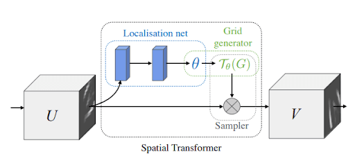
Localization network: This network takes in the input feature map U of width W, height H, and channels C. Its job is to output , the transformation parameters to be applied to the feature map.

The localization network can be anything: A fully connected network or a convolutional network. The only important thing is that it has to contain a final regression layer, which outputs .

Parameterized Sampling Grid: We have the parameters of transformation . Let’s assume our input feature map to be U, as shown in Figure 4. We can see that U is a rotated version of the number 9. Our output feature map V is a square grid. Hence we already know its indices (i.e., a normal rectangular grid).

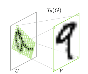
While the transformation can be anything, let us assume that our input feature requires an affine transformation.

The transformation grid gives us: . Let’s understand what this means. The matrix U is our input feature map. For each of its source coordinates, we are defining it as the transformation matrix multiplied by each of the target coordinates from the output feature map V.

So, to sum up, the matrix maps the output pixel coordinates back to the source pixel coordinates.

But in the end, these are just coordinates. How will we know the values in these pixels? For that, we will move on to the sampler.

Sampler: Now that we have our coordinates, the output feature map V values will just be estimated using our input pixel values. That is, we will perform a linear/bilinear interpolation of the output pixels using the input pixels. Bilinear interpolation uses the nearest pixel values, which are located in diagonal directions from a given location, in order to find the appropriate color intensity values of that pixel.

We’ll address each of these modules separately as we go through the code.

---

Configuring Your Development Environment

To follow this guide, you need to have the OpenCV library installed on your system.

Luckily, OpenCV is pip-installable:

$ pip install tensorflow
$ pip install matplotlib

If you need help configuring your development environment for OpenCV, we highly recommend that you read our pip install OpenCV guide — it will have you up and running in a matter of minutes.

---

Having Problems Configuring Your Development Environment?

All that said, are you:

• Short on time?
• Learning on your employer’s administratively locked system?
• Wanting to skip the hassle of fighting with the command line, package managers, and virtual environments?
• Ready to run the code right now on your Windows, macOS, or Linux system?

Then join PyImageSearch University today!

Gain access to Jupyter Notebooks for this tutorial and other PyImageSearch guides that are pre-configured to run on Google Colab’s ecosystem right in your web browser! No installation required.

And best of all, these Jupyter Notebooks will run on Windows, macOS, and Linux!

---

Project Structure

We first need to review our project directory structure.

Start by accessing the “Downloads” section of this tutorial to retrieve the source code and example images.

From there, take a look at the directory structure:

!tree .
.
├── create_gif.py
├── pyimagesearch
│   ├── callback.py
│   ├── classification_model.py
│   ├── config.py
│   └── stn.py
├── stn.gif
└── train.py

1 directory, 7 files

The create_gif.py script will help us create a gif out of the output images.

Inside the pyimagesearch directory, we have 4 scripts:

• callback.py: Contains callbacks to be used during model training.
• classification_model.py: Contains the base model to be used for training.
• config.py: Contains the end-to-end configuration pipeline of the project.
• stn.py: Contains the definition of the spatial transformer block.

In the core directory, we have train.py, where the model training occurs, and the stn.gif, which is our output gif.

---

Preparing the Configuration Script

Before starting the implementation, let’s hop into the config.py script inside the pyimagesearch directory. This script will have defined global variables and paths used throughout the project.

# import the necessary packages
from tensorflow.data import AUTOTUNE
import os

# define AUTOTUNE
AUTO = AUTOTUNE

# define the image height, width and channel size
IMAGE_HEIGHT = 28
IMAGE_WIDTH = 28
CHANNEL = 1

# define the dataset path, dataset name, and the batch size
DATASET_PATH = "dataset"
DATASET_NAME = "emnist"
BATCH_SIZE = 1024

On Line 6, we have defined the AUTOTUNE feature of tensorflow.data. This way, the runtime values (related allocation of parameters across CPU) for a tfds will be dynamically optimized to benefit the user.

Next, we define our input images’ height, width, and channel values (Lines 9-11). Since we will be using black and white images, our channel value is 1.

On Line 14, we have defined a dataset path, followed by specifying which dataset we want in our project (Line 15). Finally, we define a value for the size of the batches our data will be split into (Line 16).

# define the number of epochs
EPOCHS = 100

# define the conv filters
FILTERS = 256

# define an output directory
OUTPUT_PATH = "output"

# define the loss function and optimizer
LOSS_FN = "sparse_categorical_crossentropy"
OPTIMIZER = "adam"

# define the name of the gif
GIF_NAME = "stn.gif"

# define the number of classes for classification
CLASSES = 62

# define the stn layer name
STN_LAYER_NAME = "stn"

Next, we define some hyperparameters like the number of epochs (Line 19) and the number of convolution filters (Line 22), followed by a reference to the output folder path (Line 25).

For today’s project, we will use sparse_categorical_crossentropy as our loss function and adam as our optimizer (Lines 28 and 29).

To visualize our output, we will be using a GIF. We have defined a reference to the GIF on Line 32. The emnist dataset has 62 classes, as defined in Line 35. It is a dataset created using the same format as the mnist dataset, but it has more complex data entries for more robust training.

For more information on this dataset, please visit the official arXiv link.

Finally, we have our spatial transformer network variable name on Line 38.

---

Implementing a Callback Function for Output GIF

This function will help us build our GIF. It will also allow us to track the progress of our model while it is training. This function can be found in the callback.py script in pyimagesearch.

# import the necessary packages
from tensorflow.keras.callbacks import Callback
from tensorflow.keras import Model
import matplotlib.pyplot as plt

def get_train_monitor(testDs, outputPath, stnLayerName):
	# iterate over the test dataset and take a batch of test images
	(testImg, _) = next(iter(testDs))

We define the function on Line 6. It takes in the following arguments:

• testDs: The test dataset
• outputPath: Folder where the images will be stored
• stnLayerName: Layer name for layerwise output

On Line 8, we use next(iter(dataset)) to iterate over our complete dataset. This is because our dataset has generator-like properties. The current batch images are stored in the testImg variable.

	# define a training monitor
	class TrainMonitor(Callback):
		def on_epoch_end(self, epoch, logs=None):
			model = Model(self.model.input,
				self.model.get_layer(stnLayerName).output)
			testPred = model(testImg)

			# plot the image and the transformed image
			_, axes = plt.subplots(nrows=5, ncols=2, figsize=(5, 10))
			for ax, im, t_im  in zip(axes, testImg[:5], testPred[:5]):
				ax[0].imshow(im[..., 0], cmap="gray")
				ax[0].set_title(epoch)
				ax[0].axis("off")

				ax[1].imshow(t_im[..., 0], cmap="gray")
				ax[1].set_title(epoch)
				ax[1].axis("off")
			
			# save the figures
			plt.savefig(f"{outputPath}/{epoch:03d}")
			plt.close()
	
	# instantiate the training monitor callback
	trainMonitor = TrainMonitor()

	# return the training monitor object
	return trainMonitor

On Line 11, we define a training monitor class, inheriting from TensorFlow’s callback module. Inside it, we have another function called on_epoch_end which will fire up after each epoch (Line 12). It takes the current epoch number and logs as its arguments.

On Lines 13 and 14, we define a mini model inside the function. This mini model takes all the layers from our main model to the spatial transformer layer since we need the output of this layer. On Line 15, we pass the current test batch through the mini model and get its output.

On Lines 18-26, we define a complete subplot system where the first 5 test images and their corresponding predictions are plotted side by side. We then save the figure to our output path (Line 29).

Before we close the function, we instantiate an object of the trainMonitor class (Line 33).

---

The Spatial Transformer Module

To attach the spatial transformer module to our main model, we have created a separate script that will contain all necessary helper functions as well as the main stn layer. So for that, let’s move to the stn.py script.

Before we get into the code, let’s briefly recap what we are trying to accomplish.

• Our input image will give us the required transformation parameters.
• We will map the input feature map from the output feature map.
• We will apply bilinear interpolation to estimate the output feature map pixel values.

If you remember these pointers, let’s analyze the code.

# import the necessary packages
from tensorflow.keras import Sequential
from tensorflow.keras.layers import Conv2D
from tensorflow.keras.layers import MaxPool2D
from tensorflow.keras.layers import GlobalAveragePooling2D
from tensorflow.keras.layers import Reshape
from tensorflow.keras.layers import Dense
from tensorflow.keras.layers import Layer
import tensorflow as tf

def get_pixel_value(B, H, W, featureMap, x, y):
	# create batch indices and reshape it
	batchIdx = tf.range(0, B)
	batchIdx = tf.reshape(batchIdx, (B, 1, 1))

	# create the indices matrix which will be used to sample the 
	# feature map
	b = tf.tile(batchIdx, (1, H, W))
	indices = tf.stack([b, y, x], 3)

	# gather the feature map values for the corresponding indices
	gatheredPixelValue = tf.gather_nd(featureMap, indices)

	# return the gather pixel values
	return gatheredPixelValue

The first important function in this script is get_pixel_value (Line 11). It takes in:

• The batch size, height, and width values
• The input feature map
• x and y coordinates of a given pixel.

This function will help you salvage the pixel value at the corner coordinates by directly accessing them from the feature map.

On Lines 13 and 14, we are creating placeholder batch indices. Next, we create an indices matrix which we will use to sample from the feature map (Lines 18 and 19). On Line 22, we get the feature map values for the corresponding coordinates using tf.gather_nd.

def affine_grid_generator(B, H, W, theta):
	# create normalized 2D grid
	x = tf.linspace(-1.0, 1.0, H)
	y = tf.linspace(-1.0, 1.0, W)
	(xT, yT) = tf.meshgrid(x, y)

	# flatten the meshgrid
	xTFlat = tf.reshape(xT, [-1])
	yTFlat = tf.reshape(yT, [-1])

	# reshape the meshgrid and concatenate ones to convert it to 
	# homogeneous form
	ones = tf.ones_like(xTFlat)
	samplingGrid = tf.stack([xTFlat, yTFlat, ones])

	# repeat grid batch size times
	samplingGrid = tf.broadcast_to(samplingGrid, (B, 3, H * W))

	# cast the affine parameters and sampling grid to float32 
	# required for matmul
	theta = tf.cast(theta, "float32")
	samplingGrid = tf.cast(samplingGrid, "float32")

	# transform the sampling grid with the affine parameter
	batchGrids = tf.matmul(theta, samplingGrid)

	# reshape the sampling grid to (B, H, W, 2)
	batchGrids = tf.reshape(batchGrids, [B, 2, H, W])

	# return the transformed grid
	return batchGrids

The next function under the microscope is affine_grid_generator on Line 27. It takes in the following arguments:

• Batch size
• Height
• Width
• Transformation parameter theta

Let’s understand what we are trying to do here. At the start of this blog, we have told you that the grid generator gives us the following formula: , where U is our input feature map and V is our output feature map.

So the step where we are mapping the output coordinates back to the input coordinates is what we are trying to accomplish here.

For that, we first create a normalized 2D grid on Lines 29-31. We then flatten and create a homogeneous grid (Lines 34-40). Notice that the variables are named xT, yT, echoing the target coordinates we explained in the first section of this tutorial.

Since we need grids equal to the batch size, we repeat the grid size on Line 43.

Our next step is the matrix multiplication between our target coordinates and the transformation parameters theta. For that, we first cast them to float (Lines 47 and 48) and then use tf.matmul to multiply them (Line 51).

Finally, we reshape the batchGrids variable and make the function return the value (Lines 54-57). Note that the reshape value is (B, 2, H, W). The value 2 is because we have to get both the X coordinate meshgrid and Y coordinate meshgrid.

def bilinear_sampler(B, H, W, featureMap, x, y):
	# define the bounds of the image
	maxY = tf.cast(H - 1, "int32")
	maxX = tf.cast(W - 1, "int32")
	zero = tf.zeros([], dtype="int32")

	# rescale x and y to feature spatial dimensions
	x = tf.cast(x, "float32")
	y = tf.cast(y, "float32")
	x = 0.5 * ((x + 1.0) * tf.cast(maxX-1, "float32"))
	y = 0.5 * ((y + 1.0) * tf.cast(maxY-1, "float32"))

	# grab 4 nearest corner points for each (x, y)
	x0 = tf.cast(tf.floor(x), "int32")
	x1 = x0 + 1
	y0 = tf.cast(tf.floor(y), "int32")
	y1 = y0 + 1

	# clip to range to not violate feature map boundaries
	x0 = tf.clip_by_value(x0, zero, maxX)
	x1 = tf.clip_by_value(x1, zero, maxX)
	y0 = tf.clip_by_value(y0, zero, maxY)
	y1 = tf.clip_by_value(y1, zero, maxY)

Moving on to our bilinear_sampler function will help us get the complete output feature map. It takes in the following arguments:

• The batch size, height, and width
• The input feature map
• The x and y coordinates obtained from the previous function affine_grid_generator

On Lines 61-63, we define the image’s bounds according to the height and width indexes.

On Lines 66-69, we are rescaling x and y to match the feature map spatial dimensions (i.e., in the interval from 0 to 400).

On Lines 72-75, we grab the 4 nearest corner points for each given x and y coordinate.

That is followed by clipping the values not to let them violate the feature map boundaries (Lines 78-81).

	# get pixel value at corner coords
	Ia = get_pixel_value(B, H, W, featureMap, x0, y0)
	Ib = get_pixel_value(B, H, W, featureMap, x0, y1)
	Ic = get_pixel_value(B, H, W, featureMap, x1, y0)
	Id = get_pixel_value(B, H, W, featureMap, x1, y1)

	# recast as float for delta calculation
	x0 = tf.cast(x0, "float32")
	x1 = tf.cast(x1, "float32")
	y0 = tf.cast(y0, "float32")
	y1 = tf.cast(y1, "float32")

	# calculate deltas
	wa = (x1-x) * (y1-y)
	wb = (x1-x) * (y-y0)
	wc = (x-x0) * (y1-y)
	wd = (x-x0) * (y-y0)

	# add dimension for addition
	wa = tf.expand_dims(wa, axis=3)
	wb = tf.expand_dims(wb, axis=3)
	wc = tf.expand_dims(wc, axis=3)
	wd = tf.expand_dims(wd, axis=3)

	# compute transformed feature map
	transformedFeatureMap = tf.add_n(
		[wa * Ia, wb * Ib, wc * Ic, wd * Id])

	# return the transformed feature map
	return transformedFeatureMap

Now that we have the corner coordinates, we grab the pixel values using the get_pixel_value function previously created. This concludes the interpolation step (Lines 84-87).

On Lines 90-93, we recast the coordinates as float for delta calculation. Finally, the deltas are calculated on Lines 96-99.

Let us understand what is going on here. First, our image will go through interpolations in some areas according to our transformation matrix. The pixel values will be averages of their corner points in those areas. But to get our actual outputs, we will need to divide our altered feature map with the actual feature map to get the desired result.

On Lines 102-109, we compute our transformed final feature map using the deltas.

class STN(Layer):
	def __init__(self, name, filter):
		# initialize the layer
		super().__init__(name=name)
		self.B = None
		self.H = None
		self.W = None
		self.C = None

		# create the constant bias initializer
		self.output_bias = tf.keras.initializers.Constant(
			[1.0, 0.0, 0.0,
			0.0, 1.0, 0.0]
		)

		# define the filter size
		self.filter = filter

Now it’s time to bring our complete setup together. We have created a class called stn on Line 114, inherited from the keras.layer class.

The __init__ function is used to initialize and assign the variables we will use in the call function (Lines 117-130). The output_bias will be used in the dense functions later.

	def build(self, input_shape):
		# get the batch size, height, width and channel size of the
		# input
		(self.B, self.H, self.W, self.C) = input_shape

		# define the localization network
		self.localizationNet = Sequential([
			Conv2D(filters=self.filter // 4, kernel_size=3,
				input_shape=(self.H, self.W, self.C), 
				activation="relu", kernel_initializer="he_normal"),
			MaxPool2D(),
			Conv2D(filters=self.filter // 2, kernel_size=3,
				activation="relu", kernel_initializer="he_normal"),
			MaxPool2D(),
			Conv2D(filters=self.filter, kernel_size=3,
				activation="relu", kernel_initializer="he_normal"),
			MaxPool2D(),
			GlobalAveragePooling2D()
		])

		# define the regressor network
		self.regressorNet = tf.keras.Sequential([
			Dense(units = self.filter, activation="relu",
				kernel_initializer="he_normal"),
			Dense(units = self.filter // 2, activation="relu",
				kernel_initializer="he_normal"),
			Dense(units = 3 * 2, kernel_initializer="zeros",
				bias_initializer=self.output_bias),
			Reshape(target_shape=(2, 3))
		])

As mentioned earlier, the localization net will give us the transformation parameters theta as output. We have split the Localization net into 2 separate parts. On Lines 138-150, we have the convolution localization net, which will give us the feature map as output.

On Lines 153-161, we have the regressor net, which takes the convolution output as its input and gives us the transformation parameters theta. Here, we can safely say that theta becomes a learnable parameter.

	def call(self, x):
		# get the localization feature map
		localFeatureMap = self.localizationNet(x)

		# get the regressed parameters
		theta = self.regressorNet(localFeatureMap)

		# get the transformed meshgrid
		grid = affine_grid_generator(self.B, self.H, self.W, theta)

		# get the x and y coordinates from the transformed meshgrid
		xS = grid[:, 0, :, :]
		yS = grid[:, 1, :, :]

		# get the transformed feature map
		x = bilinear_sampler(self.B, self.H, self.W, x, xS, yS)

		# return the transformed feature map
		return x

Finally, we come to the call function (Line 163). Here, we first create the feature map on Line 165, passing it through the regressorNet and getting our transformation parameters (Line 168).

Now that we have theta, we can create our grid using the affine_grid_generator function on Line 171. Now we can separate the x and y source coordinates from our grid by indexing them and passing them through our bilinear sampler (Lines 174-178).

---

The Classification Model

Our complete classification model is relatively simple since we have already created the spatial transformer module. So let’s move on to the classification_model.py script and analyze the architecture.

# import the necessary packages
from tensorflow.keras import Input
from tensorflow.keras import Model
from tensorflow.keras.layers import Conv2D
from tensorflow.keras.layers import MaxPool2D
from tensorflow.keras.layers import Reshape
from tensorflow.keras.layers import GlobalAveragePooling2D
from tensorflow.keras.layers import Lambda
from tensorflow.keras.layers import Dense
from tensorflow.keras.layers import Dropout
import tensorflow as tf


def get_training_model(batchSize, height, width, channel, stnLayer,
	numClasses, filter):
	# define the input layer and pass the input through the STN
	# layer
	inputs = Input((height, width, channel), batch_size=batchSize)
	x = Lambda(lambda image: tf.cast(image, "float32")/255.0)(inputs)
	x = stnLayer(x) 

Our main training model is obtained using the function get_training_model on Line 14. It takes in the following arguments:

• Batch size, height, width, and channel values
• The spatial transformer layer
• The number of output classes and the number of filters

On Line 18, we initialize the model input. Next, we scale the image to 0 and 1 (Line 19).

We proceed to add the spatial transformer layer next, on Line 20. The perk of creating a module is that our main architecture script is much less cluttered.

	# apply a series of conv and maxpool layers
	x = Conv2D(filter // 4, 3, activation="relu", 
		kernel_initializer="he_normal")(x)
	x = MaxPool2D()(x)
	x = Conv2D(filter // 2, 3, activation="relu",
		kernel_initializer="he_normal")(x)
	x = MaxPool2D()(x)
	x = Conv2D(filter, 3, activation="relu",
		kernel_initializer="he_normal")(x)
	x = MaxPool2D()(x)

	# global average pool the output of the previous layer
	x = GlobalAveragePooling2D()(x)

	# pass the flattened output through a couple of dense layers
	x = Dense(filter, activation="relu",
		kernel_initializer="he_normal")(x)
	x = Dense(filter // 2, activation="relu",
		kernel_initializer="he_normal")(x)

	# apply dropout for better regularization
	x = Dropout(0.5)(x)

	# apply softmax to the output for a multi-classification task
	outputs = Dense(numClasses, activation="softmax")(x)

	# return the model
	return Model(inputs, outputs)

The rest of the layers are pretty straightforward. On Lines 23-31, we have repeating sets of a Conv2D layer and a Max pooling layer.

This is followed by a global average pooling layer on Line 34.

We add two dense layers followed by a dropout layer before finally adding our output layer to give us a softmax over the number of classes (Lines 37-46).

The function then returns an initialized model (Line 49).

---

Training the Model

With all configuration pipelines, helper functions, and model architectures completed, we just need to plug the data in and see the results. For that, let’s move on to train.py.

# USAGE
# python train.py

# setting seed for reproducibility
import tensorflow as tf
tf.random.set_seed(42)

# import the necessary packages
from pyimagesearch.stn import STN
from pyimagesearch.classification_model import get_training_model
from pyimagesearch.callback import get_train_monitor
from pyimagesearch import config
from tensorflow.keras.callbacks import EarlyStopping
import tensorflow_datasets as tfds
import os

# load the train and test dataset
print("[INFO] loading the train and test dataset...")
trainingDs = tfds.load(name=config.DATASET_NAME,
	data_dir=config.DATASET_PATH, split="train", shuffle_files=True,
	as_supervised=True)
testingDs = tfds.load(name=config.DATASET_NAME,
	data_dir=config.DATASET_PATH, split="test", as_supervised=True)

It’s important to remember to call our scripts in the imports section (Lines 5-15). Next, we use tfds.load to directly download our required dataset (Lines 19-23). We do this to get both training and test splits.

 # preprocess the train and test dataset
print("[INFO] preprocessing the train and test dataset...")
trainDs = (
	trainingDs
	.shuffle(config.BATCH_SIZE*100)
	.batch(config.BATCH_SIZE, drop_remainder=True)
	.prefetch(config.AUTO)
)
testDs = (
	testingDs
	.batch(config.BATCH_SIZE, drop_remainder=True)
	.prefetch(config.AUTO)
)

# initialize the stn layer
print("[INFO] initializing the stn layer...")
stnLayer = STN(name=config.STN_LAYER_NAME, filter=config.FILTERS)

# get the classification model for cifar10
print("[INFO] grabbing the multiclass classification model...")
model = get_training_model(batchSize=config.BATCH_SIZE,
	height=config.IMAGE_HEIGHT, width=config.IMAGE_WIDTH,
	channel=config.CHANNEL, stnLayer=stnLayer,
	numClasses=config.CLASSES, filter=config.FILTERS)

Once we have our training and testing datasets, we preprocess them on Lines 27-37.

On Line 41, we initialize a Spatial transformer module layer using the scripts and configuration variables we have created beforehand.

Then we initialize our main model by passing the stn layer along with the required configuration variables (Lines 45-48).

# print the model summary
print("[INFO] the model summary...")
print(model.summary())

# create an output images directory if it not already exists
if not os.path.exists(config.OUTPUT_PATH):
	os.makedirs(config.OUTPUT_PATH)

# get the training monitor
trainMonitor = get_train_monitor(testDs=testDs,
	outputPath=config.OUTPUT_PATH, stnLayerName=config.STN_LAYER_NAME)

# compile the model
print("[INFO] compiling the model...")
model.compile(loss=config.LOSS_FN, optimizer=config.OPTIMIZER, 
	metrics=["accuracy"])

# define an early stopping callback
esCallback = EarlyStopping(patience=5, restore_best_weights=True)

# train the model
print("[INFO] training the model...")
model.fit(trainDs, epochs=config.EPOCHS, 
	callbacks=[trainMonitor, esCallback], validation_data=testDs)

For a sanity check, we display the model summary on Line 52.

Next, we create an output directory using os.makedirs on Lines 55 and 56.

Since our model has been created, we initialize the callback script’s object trainMonitor on Lines 59 and 60. To recap, this will give us visualizations of how our training affects our test dataset’s outputs.

We then compile the model with our configuration variables and choose accuracy as our metric (Lines 64 and 65).

For efficiency’s sake, we define an early stopping callback function on Line 68. This will stop the model training if a moderate accuracy value has been reached.

On Lines 72 and 73, we end the script by fitting our dataset and callbacks into our model and starting the training step.

---

Model Training and Visualizations

Let’s see how well our model training fared!

[INFO] compiling the model...
[INFO] training the model...
Epoch 1/100
681/681 [==============================] - 104s 121ms/step - loss: 0.9146 - accuracy: 0.7350 - val_loss: 0.4381 - val_accuracy: 0.8421
Epoch 2/100
681/681 [==============================] - 84s 118ms/step - loss: 0.4705 - accuracy: 0.8392 - val_loss: 0.4064 - val_accuracy: 0.8526
Epoch 3/100
681/681 [==============================] - 85s 119ms/step - loss: 0.4258 - ... 
Epoch 16/100
681/681 [==============================] - 85s 119ms/step - loss: 0.3192 - accuracy: 0.8794 - val_loss: 0.3483 - val_accuracy: 0.8725
Epoch 17/100
681/681 [==============================] - 85s 119ms/step - loss: 0.3151 - accuracy: 0.8803 - val_loss: 0.3487 - val_accuracy: 0.8736
Epoch 18/100
681/681 [==============================] - 85s 118ms/step - loss: 0.3113 - accuracy: 0.8814 - val_loss: 0.3503 - val_accuracy: 0.8719

As we can see, by epoch 18, the early stopping came into effect and stopped the model training. As a result, the final training and validation accuracies are 88.14% and 87.19%, respectively.

Let’s see some visualizations in Figure 6.

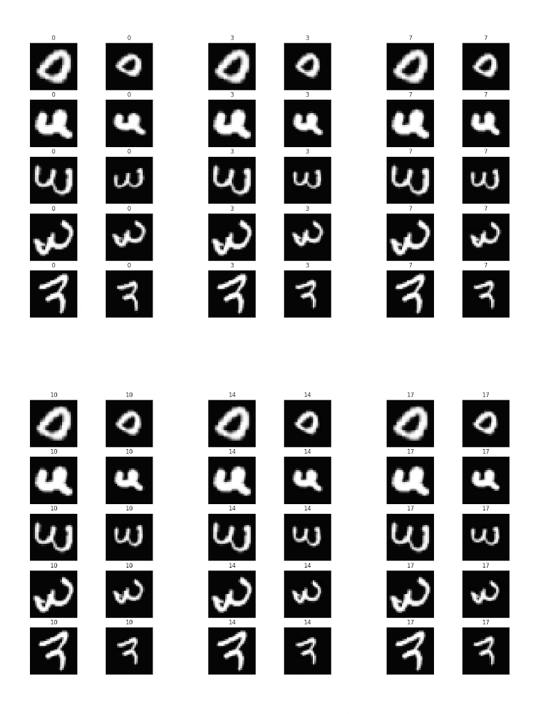
In Figure 6, we can see a batch of digits getting transformed in each epoch. You might notice that the transformations aren’t very understandable to the human eye.

However, you have to keep in mind that the transformation won’t always happen based on how the digits look to us. It depends on which transformation gets the loss lower. So it might not be something that we understand, but if it works for the loss function, it’s good enough for the model!

---

---

Summary

Transformational invariance is a highly relevant factor in today’s deep learning world. Vision tasks employ the use of deep learning in some form or another. When real-life factors are at stake, it is important to create robust and built systems to handle as many scenarios as possible.

Our results have shown that the system works in unison; Backpropagation gives us the correct transformation parameters while the initial grid starts fixing itself with each epoch.

If you think about it, we identify a digit from an image, while the whole picture is important for a deep learning system. So If it can identify the exact pixels to work with, it is definitely more efficient.

Convolutional Networks possessing transformational invariance really help build towards the goal of robust Artificial Intelligence (AI) systems. The added benefit is that we take a step closer to making AI systems closer to the human brain.

The popularity of attachable modules for CNN has recently risen. You can catch next week’s blog on Attending to feature map channels, which uses another attachable module to better your model.

---

Credits

This tutorial was inspired by the works of Sayak Paul and Kevin Zakka.

---

Citation Information

Chakraborty, D. “Spatial Transformer Networks Using TensorFlow,” PyImageSearch, P. Chugh, A. R. Gosthipaty, S. Huot, K. Kidriavsteva, R. Raha, and A. Thanki, eds., 2022, https://pyimg.co/4ham6

@incollection{Chakraborty_2022_Spatial_Transformer,
  author = {Devjyoti Chakraborty},
  title = {Spatial Transformer Networks Using {TensorFlow}},
  booktitle = {PyImageSearch},
  editor = {Puneet Chugh and Aritra Roy Gosthipaty and Susan Huot and Kseniia Kidriavsteva and Ritwik Raha and Abhishek Thanki},
  year = {2022},
  note = {https://pyimg.co/4ham6},
}

---

To download the source code to this post (and be notified when future tutorials are published here on PyImageSearch), simply enter your email address in the form below!