Mean Average Precision (mAP) Using the COCO Evaluator

---

---

Mean Average Precision (mAP) Using the COCO Evaluator

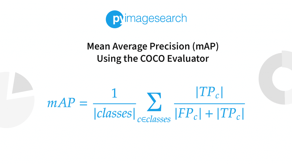
In this tutorial, you will learn Mean Average Precision (mAP) in object detection and evaluate a YOLO object detection model using a COCO evaluator.

This is the 4th lesson in our 7-part series on the YOLO Object Detector:

1. Introduction to the YOLO Family
2. Understanding a Real-Time Object Detection Network: You Only Look Once (YOLOv1)
3. A Better, Faster, and Stronger Object Detector (YOLOv2)
4. Mean Average Precision (mAP) Using the COCO Evaluator (today’s tutorial)
5. An Incremental Improvement with Darknet-53 and Multi-Scale Predictions (YOLOv3)
6. Achieving Optimal Speed and Accuracy in Object Detection (YOLOv4)
7. Training the YOLOv5 Object Detector on a Custom Dataset

We will discuss these key topics in this post:

• What are Precision and Recall?
• The Precision-Recall (PR) curve
• Intersection over Union (IoU)
• Average Precision (AP)
• Mean Average Precision (mAP)
• Walk through the code implementation of evaluating a YOLO object detection model using a COCO evaluator

Before we get started, are you familiar with how an object detector works, especially a single-stage detector like YOLO?

If not, be sure to look at our previous posts, Introduction to the YOLO Family and Understanding a Real-Time Object Detection Network: You Only Look Once (YOLOv1), for a high-level intuition of how a single-stage object detection works in general. Single-Stage Object Detectors treat object detection as a simple regression problem. For example, the input image fed to the network directly outputs the class probabilities and bounding box coordinates.

These models skip the region proposal stage, also known as Region Proposal Network, which is generally part of Two-Stage Object Detectors that are areas of the image that could contain an object.

To learn what is mAP in object detection and how to evaluate an object detection model using a COCO evaluator, just keep reading.

---

Mean Average Precision (mAP) Using the COCO Evaluator

When solving a problem involving machine learning and deep learning, we usually have various models to choose from; for example, in image classification, one could select VGG16 or ResNet50. Each one has its peculiarities and would perform differently based on various factors like the dataset or target platform. And to finally decide on the best model by objectively comparing models for our use case, we need to have an evaluation metric in place.

After the model is trained or fine-tuned on the training set, it is then judged by how well or accurately it performs over the validation and test data. Various evaluation metrics or statistics could evaluate the deep learning models, but which metric to use depends on the particular problem statement and application.

The most common metric used for evaluation in an image classification problem is Precision, Recall, Confusion-matrix, PR-curve, etc. While in image segmentation, Mean Intersection over Union, aka mIoU, is used.

However, if we address the elephant in the room, the most common metric of choice used for Object Detection problems is Mean Average Precision (aka mAP).

Since in object detection, the objective is not only to correctly classify the object (or objects) in the image but to also find where in the image it is located, we cannot simply use the image classification metrics like Precision and Recall.

Hence, the object detection evaluation metric needs to consider both the category and location of the objects in its formulation, and that’s where mAP comes into play. And to understand mAP, it is necessary to understand IoU, Precision, Recall, and Precision-Recall curve. So let’s dig right into it!

---

Configuring Your Development Environment

To follow this guide, you need to have the Pycocotools library installed on your system. For additional image handling purposes, you’ll be using OpenCV, Sklearn for computing Precision and Recall, Matplotlib for plotting graphs, and a few more libraries.

Luckily, all the libraries below are pip-installable!

$ pip install pycocotools==2.0.4
$ pip install matplotlib==3.2.2
$ pip install opencv==4.1.2
$ pip install progressbar==3.38.0
$ pip install sklearn==1.0.2

That is all for the environment configuration necessary for this guide!

However, you will also need to install the Darknet framework on your system to run an inference with YOLOv4. For that, we would highly recommend you check out AlexeyAB’s Darknet Repository.

---

Having Problems Configuring Your Development Environment?

All that said, are you:

• Short on time?
• Learning on your employer’s administratively locked system?
• Wanting to skip the hassle of fighting with the command line, package managers, and virtual environments?
• Ready to run the code right now on your Windows, macOS, or Linux system?

Then join PyImageSearch University today!

Gain access to Jupyter Notebooks for this tutorial and other PyImageSearch guides that are pre-configured to run on Google Colab’s ecosystem right in your web browser! No installation required.

And best of all, these Jupyter Notebooks will run on Windows, macOS, and Linux!

---

Project Structure

Before we get into the theory and implementation of various key topics, let’s look at the project structure.

Once we have downloaded our project directory, it should look like this:

$ tree .
.
├── darknet
├── data
│   ├── dog.jpg
│   ├── label2idx.pkl
│   └── yolo_90_class_map.pkl
├── eval_iou.py
├── eval_map.py
├── main.py
├── pyimagesearch
│   ├── __init__.py
│   ├── config.py
│   ├── utils_iou.py
│   ├── utils_map.py
│   └── utils_precision_recall.py
└── results
    ├── COCO_Val_mAP.png
    ├── dog_iou.png
    └── pr_curve.png

36 directories, 2135 files

Please note that we do not show the darknet directory since it has a lot of files, and it would be difficult to put all the files as part of the directory structure.

The parent directory has 3 python scripts and 4 folders.

• main.py: This is the driver script that is the entry point to our experiments. Based on the command line input received from the user, it will execute one of three experiments (IoU, Precision-Recall Curve, or COCO Evaluator).

• eval_iou.py: The python script has the compute_iou() method. It is called from the main. It takes imagePath as a parameter and calls two methods: first to compute IoU and second to display the output on the screen.

• eval_map.py: It loads the ground-truth annotation file, calls the run_inference() method to generate the predictions, and then computes mAP and displays the results on the terminal.

Next, let’s get into the pyimagesearch directory! In it, we will find 5 python scripts:

• __init__.py: This will make Python treat the pyimagesearch directory as a module
• config.py: This script contains various hyperparameter presets and defines the data paths
• utils_iou.py: This script has the implementation of the IoU method and plot method
• utils_map.py: This script contains an image_detection method that runs inference per image, a few methods for loading pickle files, and modifying bounding box coordinates. It also has the run_inference() method that iterates over each image calls image_detection() and stores the prediction in JSON format
• utils_precision_recall.py: This script has a bunch of methods for compute precision, recall over various thresholds, and a method to plot the precision-recall curve

Next, we have the data directory, which contains:

• Sample image on which we will run the IoU experiment
• Pickle files that store object category related information
• We will download the YOLOv4 weight in this directory
• Finally, we will also download the MS COCO validation images and ground-truth annotations here

Lastly, we have the results directory, which contains:

• COCO_Val_mAP.png: The YOLOv4 mAP results on the COCO validation dataset
• dog_iou.png: A sample IoU output on the dog image
• pr_curve.png: The Precision-Recall curve plot

---

Intersection over Union (IoU)

Intersection over Union, also known as Jaccard Index, measures the overlap between the ground-truth bounding boxes and the predicted bounding boxes. It is the ratio between the Intersection and Union of the ground truth boxes with the predicted bounding boxes. The ground-truth bounding boxes are the hand-labeled bounding boxes from the testing set that specify wherein the image of our object is and the predicted bounding boxes come from the model.

As long as we have these two (ground-truth and prediction) bounding boxes, we can apply Intersection over Union.

Figure 2 is a visual example of a ground-truth bounding box versus a predicted bounding box. The goal is to compute the Intersection over Union between these two bounding boxes.

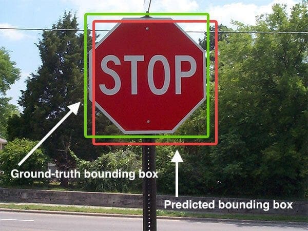
In Figure 2, we can see that the object detector has detected the presence of a stop sign in an image. The predicted bounding box is drawn in red, while the ground-truth (i.e., hand-labeled) bounding box is drawn in green.

As shown in Figure 3, Intersection over Union is as simple as dividing the area of overlap between the bounding boxes by the area of union.

From Figure 3, you can see that Intersection over Union is simply a ratio. In the numerator, we compute the area of overlap between the predicted bounding box and the ground-truth bounding box.

The denominator is the area of union or the area encompassed by the predicted bounding box and the ground-truth bounding box.

The IoU score is normalized (since the denominator is the union area), ranging from 0.0 to 1.0. Here 0.0 represents no overlap between the predicted and ground-truth bounding box, while 1.0 is the most optimal, meaning the predicted bounding box fully overlaps the ground-truth bounding box.

An Intersection over Union score > 0.5 is typically considered a “good” prediction.

---

Why Do We Use IoU?

Suppose you have performed any previous machine learning in your career, specifically classification. In that case, you’ll likely be used to predicting class labels where your model outputs a single label that is either correct or incorrect.

This type of binary classification makes computing accuracy straightforward; however, it’s not so simple for object detection.

In reality, it’s implausible that the (x, y)-coordinates of our predicted bounding box will exactly match the (x, y)-coordinates of the ground-truth bounding box.

Due to varying parameters of our model (image pyramid scale, sliding window size, feature extraction method, etc.), a complete and total match between predicted and ground-truth bounding boxes is simply unrealistic.

Because of this, we need to define an evaluation metric that rewards predicted bounding boxes for heavily overlapping (not 100%) with the ground truth.

Figure 4 shows examples of good and bad Intersection over Union scores; the IoU scores demonstrated in each case are just for intuition purposes and might not be precise.

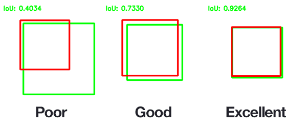
As you can see, predicted bounding boxes that heavily overlap with the ground-truth bounding boxes have higher scores than those with less overlap. This makes Intersection over Union an excellent metric for evaluating custom object detectors.

We aren’t concerned with an exact match of (x, y)-coordinates, but we want to ensure that our predicted bounding boxes match as closely as possible — Intersection over Union can take this into account.

And soon, you will see how the concept and magic of IoU benefit the mAP metric in an object detection model.

Before diving into the implementations of IoU, Precision-Recall Curve, and Evaluating YOLOv4 object detector, let’s set up our paths and hyperparameters. For that, we will hop into the module config.py. Most other scripts in our project will call this module and use its presets.

# import the necessary packages
from glob import glob

YOLO_CONFIG = "darknet/cfg/yolov4.cfg"
YOLO_WEIGHTS = "data/yolov4.weights"
COCO_DATA = "darknet/cfg/coco.data"

YOLO_NETWORK_WIDTH = 608
YOLO_NETWORK_HEIGHT = 608

LABEL2IDX = "data/label2idx.pkl"
YOLO_90CLASS_MAP = "data/yolo_90_class_map.pkl"

IMAGES_PATH = glob("data/val2017/*")

COCO_GT_ANNOTATION = "data/annotations/instances_val2017.json"
COCO_VAL_PRED = "data/COCO_Val_Predictions.json"

CONF_THRESHOLD = 0.25

IOU_GT = [90, 80, 250, 450]
IOU_PRED = [100, 100, 220, 400]

IOU_RESULT = "results/dog_iou.png"
PR_RESULT = "results/pr_curve.png"

GROUND_TRUTH_PR = ["dog", "cat", "cat", "dog", "cat", "cat", "dog",
  "dog", "cat", "dog", "dog", "dog", "dog", "cat", "cat", "dog"]
PREDICTION_PR = [0.7, 0.3, 0.5, 0.6, 0.3, 0.35, 0.55, 0.2, 0.4, 0.3,
  0.7, 0.5, 0.8, 0.2, 0.9, 0.4]

In the above lines of code, we first import the glob module (on Line 2), which is used to get all the images path as listed on Line 14.

From Lines 4-6, we define the YOLOv4 model weights and configuration file and also the COCO data file. Then we define the YOLOv4 model input width and height (i.e., 608).

Then, on Lines 11 and 12, we define the pickle file paths. The COCO ground-truth annotations and prediction JSON file paths are declared on Lines 16 and 17. The YOLOv4 confidence threshold is specified on Line 19, which is set to 0.25.

On Lines 21-24, the IoU ground-truth and prediction box coordinates are defined along with the IoU result path.

Finally, from Lines 25-30, the Precision-Recall curve experiment-related parameters are defined.

---

Coding IoU in Python

Now that we understand what Intersection over Union is and why we use it to evaluate object detection models, let’s go ahead and implement it in the utils_iou.py script. Please note that we do not run an object detector to get the predicted bounding box coordinates for the IoU example; we assume predicted coordinates. For the ground-truth coordinates, we manually annotated the image.

# import the necessary packages
from matplotlib import pyplot as plt
import cv2

def intersection_over_union(gt, pred):
    # determine the (x, y)-coordinates of the intersection rectangle
    xA = max(gt[0], pred[0])
    yA = max(gt[1], pred[1])
    xB = min(gt[2], pred[2])
    yB = min(gt[3], pred[3])

    # if there is no overlap between predicted and ground-truth box
    if xB < xA or yB < yA:
        return 0.0

    # compute the area of intersection rectangle
    interArea = max(0, xB - xA + 1) * max(0, yB - yA + 1)

    # compute the area of both the prediction and ground-truth
    # rectangles
    boxAArea = (gt[2] - gt[0] + 1) * (gt[3] - gt[1] + 1)
    boxBArea = (pred[2] - pred[0] + 1) * (pred[3] - pred[1] + 1)

    # compute the intersection over union by taking the intersection
    # area and dividing it by the sum of prediction + ground-truth
    # areas - the intersection area
    iou = interArea / float(boxAArea + boxBArea - interArea)

    # return the intersection over union value
    return iou

We begin with the necessary imports in Lines 2 and 3.

On Line 5, we define the intersection_over_union method, which requires two parameters: gt and pred are presumed to be our ground-truth and predicted bounding boxes (the actual order you supply these two parameters to intersection_over_union does not matter).

Then, from Lines 7-10, we determine the (x, y)-coordinates of the intersection rectangle, which are then used to compute the intersection area on Line 17.

On Lines 13 and 14, we perform a sanity check that if there is zero overlap between the predicted and ground-truth bounding box, then we return zero.

The inter_Area variable represents the numerator in the Intersection over Union formula.

To compute the denominator (i.e., the union area), we first need to derive the area of the predicted bounding box and the ground-truth bounding box (Lines 21 and 22).

Note: Since we are working in a “pixel coordinate space” to calculate the area of the rectangle, we must add 1 in each direction. The first pixel would start from 0 till (height/width 1) in the pixel space. For example, if an image has a width of 1920, the pixels would start from 0 and go till 1919, which would result in an incorrect area. Hence, we add 1 to the intersection and union areas calculation.

The Intersection over Union can then be computed on Line 27 by dividing the intersection area by the union area of the two bounding boxes, taking care to subtract out the intersection area from the denominator (otherwise, the intersection area would be counted twice).

Finally, the Intersection over Union score is returned to the calling function on Line 30.

def plt_imshow(title, image, path):
    # convert the image frame BGR to RGB color space and display it
    image = cv2.cvtColor(image, cv2.COLOR_BGR2RGB)
    plt.imshow(image)
    plt.title(title)
    plt.grid(False)
    plt.axis("off")
    plt.imsave(path, image)
    plt.show()

From Lines 32-40, we define the plt_imshow method that accepts two arguments: the plot’s title and the image to be displayed. And it displays the output image using the plt.show() method. Since the matplotlib plot function expects the image to be in the RGB color space, we convert the image from BGR to RGB on Line 34.

Once we have written the method for computing Intersection over Union, it is time to wrap everything together in a compute_iou method where we will pass the imagePath on which we compute the IoU, so let’s get into the eval_iou.py script.

# import the necessary packages
from pyimagesearch.utils_iou import intersection_over_union
from pyimagesearch.utils_iou import plt_imshow
from pyimagesearch import config
import cv2

def compute_iou(imagePath):
    # load the image
    image = cv2.imread(imagePath)

    # define the top-left and bottom-right coordinates of ground-truth
    # and prediction
    groundTruth = [90, 80, 250, 450]
    prediction = [100, 100, 220, 400]

    # draw the ground-truth bounding box along with the predicted
    # bounding box
    cv2.rectangle(image, tuple(groundTruth[:2]),
        tuple(groundTruth[2:]), (0, 255, 0), 2)
    cv2.rectangle(image, tuple(prediction[:2]),
        tuple(prediction[2:]), (0, 0, 255), 2)

    # compute the intersection over union and display it
    iou = intersection_over_union(groundTruth, prediction)
    cv2.putText(image, "IoU: {:.4f}".format(iou), (10, 34),
        cv2.FONT_HERSHEY_SIMPLEX, 1.4, (0, 255, 0), 3)

    # show the output image
    plt_imshow("Image", image, config.IOU_RESULT)

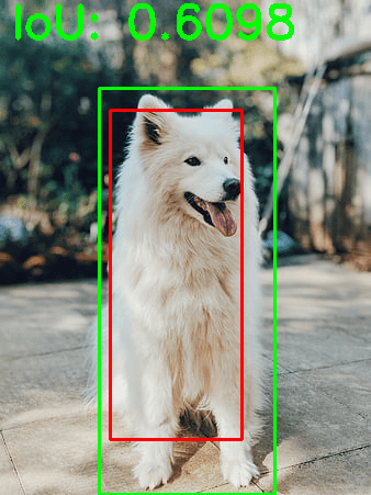
On Line 9, we load the image from the disk and then draw the ground-truth bounding box in green (Lines 18 and 19), followed by the predicted bounding box in red (Lines 20 and 21).

The Intersection over Union metric is computed on Line 24 by passing in the ground-truth and predicted bounding box coordinates that we defined on Lines 13 and 14.

We then write the Intersection over Union value on the image (Lines 25 and 26), and finally, the output image is displayed on our screen (Line 29).

In Figure 5, we can see that the Intersection over Union score is 0.6098, indicating a significant overlap between the ground-truth (green) and predicted (red) bounding box.

---

Precision and Recall

This section will discuss the precision, recall, and precision-recall curve. Since you are in the object detections series, I am sure that most of you would have worked on image classification problems earlier and would already be familiar with precision, recall, and confusion matrix and not feel alienated by these technical terms.

However, let’s recap these terms.

Imagine working on a binary classification problem in which each input sample is assigned to one of the two classes, that is, 1 (positive) and 0 (negative). For example, these two class labels could be spam or no-spam, malignant or benign (medical imaging – cancer classification problem), a simple cat or dog classifier, etc.

Let’s take an example to understand it in more detail. Assume we have a dataset with ten images of cats and others. We need to classify given an input sample where the class belongs. This means that it’s a binary classification problem.

Here we have the ground-truth labels of the data:

[cat, cat, others, cat, others, others, cat, cat, cat, others]

These class labels are currently in human-readable form; however, the model expects the ground truth to be numeric or integer. Therefore, when input is fed to the model, the model returns a score for each class. For example, the prediction of the model given the ten images from the dataset would be:

[0.8, 0.1, 0.5, 0.9, 0.28, 0.35, 0.7, 0.4, 0.2, 0.68]

Now we have the prediction from the model for each sample; for a binary classification problem, we can convert these prediction scores into class labels using a threshold. The threshold is a hyperparameter where you can experiment. For now, let’s assume the threshold to be 0.5, which means if the model predicts above or equal to 0.5, then the sample belongs to a cat (positive) class; otherwise, it is others (negative) class.

After converting the prediction into class labels using the threshold, the predicted labels would look like this:

prediction: [cat, others, cat, cat, others, others, cat, others, others, cat]

If we compare both the ground-truth and predicted labels, we can see that there are five correct and five incorrect predictions made by the model at a threshold of 0.5, and varying the threshold would alter the results.

Comparing the ground truth directly with prediction is fine, but what if we need a more in-depth analysis of our model’s performance?

For example, given a cat image, how many times does the model predict it as a cat or misclassify it as others? Similarly, for other class images, the number of times the model correctly predicted as others and misclassified as a cat.

Based on the above example, let’s define four new terms:

1. True Positive (TP): The number of times the model correctly predicted the positive input sample (i.e., cat) as Positive.
2. False Positive (FP): The number of times the model incorrectly predicted the negative sample (i.e., others) as Positive.
3. True Negative (TN): The number of times the model correctly predicted the negative sample (i.e., others) as Negative.
4. False Negative (FN): The number of times the model incorrectly predicted the positive input (i.e., cat) as Negative.

The above four terms help us extract deeper information about our model’s performance. Finally, let’s put them together to obtain Precision and Recall.

---

Precision

It is the ratio between the correctly classified Positive samples to the total number of samples classified as Positive (incorrect and correct). In short, Precision answers the question of how accurate the guesses were when the model guessed, or it measures the precision/accuracy of the model in classifying samples as positive.

In Precision, the focus is also on the Negative samples incorrectly classified as Positive since it has False Positive in its calculation. For example,

• a patient with no sign of cancer is predicted as cancer or
• a patch of an image detected as a person while there is no person in that patch

Precision can be calculated as

where are the total predicted objects.

For Precision to be high, the numerator needs to be higher (simple math). Precision would be high when the model correctly predicts the Positive samples as Positive (i.e., maximizing True Positive), and simultaneously, fewer (incorrect) Negative samples as Positive (i.e., minimizing False Positive).

The Precision would be low when the model predicts many Negative samples as Positive or fewer correct Positive classifications. This would increase the denominator and make the Precision smaller.

Now, let’s compute Precision in just a few lines of Python code.

import sklearn.metrics

ground_truth = ["cat", "cat", "others", "cat", "others", "others","cat", "cat", "cat", "others" ]
prediction = ["cat", "others", "cat", "cat", "others", "others","cat", "others", "others", "cat"]

precision = sklearn.metrics.precision_score(ground_truth, prediction, pos_label="cat")
print(precision)

In the above lines of code, we use the sklearn.metrics method to compute Precision on the cat and others examples we took above to understand the binary classification problem.

It’s relatively straightforward, from Lines 3 and 4, we define ground_truth and prediction in a list. Then pass them to the precision_score method of sklearn on Line 6. We also give a pos_label argument that lets you specify which class should be considered as positive for the Precision computation.

---

Recall

It is the ratio between the correctly classified Positive samples to the total number of actual Positive samples. Recall answers whether your model guessed every time that it should be guessing. The higher the recall, the more positive samples are detected.

where are the total ground-truth objects.

As we learned, Precision does consider how the negative samples are classified; however, Recall is independent of how the negative examples are classified and only cares about how the positive samples are classified. This means that even if all the Negative samples are classified as Positive, the Recall would still be a perfect 1.0.

The Recall would be 1.0 or 100% when all positive samples are classified as Positive. On the other hand, Recall would be low if Positive samples are classified as Negative; for example, imagine there are five cars in an image, and only four are detected, so False Negatives would be one.

import sklearn.metrics

ground_truth = ["cat", "cat", "others", "cat", "others", "others","cat", "cat", "cat", "others"]
prediction = ["cat", "others", "cat", "cat", "others", "others", "cat", "others", "others", "cat"]

recall = sklearn.metrics.recall_score(ground_truth, prediction, pos_label="cat")
print(recall)

Similar to Precision, we can calculate Recall by just changing the sklearn.metrics.precision_score to sklearn.metrics.recall_score on Line 6.

---

TP, FP, TN, and FN in Detection Context

We learned about Precision and Recall, and to calculate them, we need to compute True Positives, True Negatives, False Positives, and False Negatives. We also learned about Intersection over Union and how it helps evaluate an object detection model’s localization error. So, let’s know about Precision and Recall in object detection context and how IoU and Confidence Score play a role.

The confidence score reflects how likely the box contains an object (objectness score) and the bounding box’s accuracy. However, if no object exists in that cell, the confidence score should be zero.

---

True Positive

A detection made by the model is considered True Positive only if it satisfies the two conditions:

• The confidence score of the predicted bounding box should be greater than the confidence threshold (a hyperparameter), which would signify that we have found the object for which we were looking.
• The IoU between the predicted bounding box and the ground-truth bounding box should be greater than the IoU threshold.

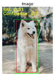
And what the above two conditions mean is that not only is the object detected, but it is detected at the correct location. Figure 6 shows the True Positive detection with an IoU of 0.81 and a Confidence of 0.7.

---

False Positive

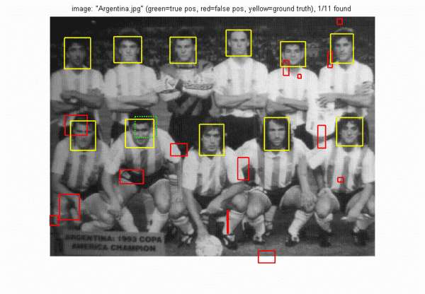
A detection is considered to be a False Positive:

• If the model detects an object with a high confidence score, but it is not present (no ground truth), then the IoU would be equal to zero.
• Another scenario could be that the IoU is less than the IoU threshold.
• If the proposed bounding box perfectly aligns with the ground truth, but the class label of the proposed box is incorrect.

---

True Negative

This is generally not required, mainly because it is not part of the computation in Precision and Recall.

A True Negative in detection could be when the confidence score is less than the confidence threshold, and also the IoU (predicted box and ground-truth box) is less than the IoU threshold. In object detection, there could be a lot of True Negatives because the background covers more areas of the image than the object itself.

---

False Negative

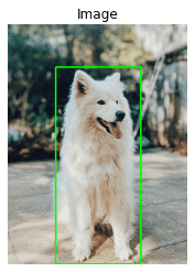
If there is an object present, but the model was not able to detect it, then that’s a False Negative.

---

Precision-Recall Curve

Based on the learnings from the previous section, we now know that if the model has both high precision and recall, then it correctly predicts the samples as positive and predicts most of the positive samples (does not miss the samples or predict them as negative). However, if the model has high precision and low recall, it accurately predicts samples as positive but only a few positive samples (more false negatives).

Now that we know the importance of precision and recall and that the ultimate goal is to achieve the maximum scores for both precision and recall, let’s see how we can plot these on the same graph.

The plotting of the precision-recall values is known as a precision-recall curve that depicts the trade-off between the two based on different thresholds. The precision-recall curve helps to select the best threshold that maximizes both precision and recall.

Let’s understand the Precision-Recall curve with a binary classification example of cat and dog. In utils_precision_recall.py, we will write the compute_precision_recall method, which will take the ground-truth and prediction vectors along with 10 threshold values in a vector. Finally, return precision and recall for each of the 10 thresholds. It will also help plot the precision-recall curve.

# import the necessary packages
from pyimagesearch import config
import matplotlib.pyplot as plt
import sklearn.metrics
import numpy as np

def compute_precision_recall(yTrue, predScores, thresholds):
    precisions = []
    recalls = []

    # loop over each threshold from 0.2 to 0.65
    for threshold in thresholds:
        # yPred is dog if prediction score greater than threshold
        # else cat if prediction score less than threshold
        yPred = [
            "dog" if score >= threshold else "cat"
            for score in predScores
        ]
  
        # compute precision and recall for each threshold
        precision = sklearn.metrics.precision_score(y_true=yTrue,
            y_pred=yPred, pos_label="dog")
        recall = sklearn.metrics.recall_score(y_true=yTrue,
            y_pred=yPred, pos_label="dog")
  
        # append precision and recall for each threshold to
        # precisions and recalls list
        precisions.append(np.round(precision, 3))
        recalls.append(np.round(recall, 3))

    # return them to calling function
    return precisions, recalls

On Line 7, we define the compute_precision_recall function, which takes the ground-truth labels, predictions scores, and threshold list as an argument.

Then, we iterate through each threshold on Line 12 convert the probabilities to a class label by checking if the prediction score (or probability) is greater than or equal to the threshold, we assign the dog label else cat.

From Lines 21-24, we compute the precision and recall for a given threshold and prediction. Then we round precision and recall to three decimal places and append them in a precisions and recalls list on Lines 28 and 29.

Finally, we return the precisions and recalls to the calling function on Line 32.

def pr_compute():
    # define thresholds from 0.2 to 0.65 with step size of 0.05
    thresholds = np.arange(start=0.2, stop=0.7, step=0.05)

    # call the compute_precision_recall function
    precisions, recalls = compute_precision_recall(
        yTrue=config.GROUND_TRUTH_PR, predScores=config.PREDICTION_PR,
        thresholds=thresholds,
    )
 
    # return the precisions and recalls
    return (precisions, recalls)

On Line 36, we define thresholds using np.arange, which creates a vector with values ranging from 0.2 to 0.65 with a step size of 0.05.

From Lines 39-42, we call the compute_precision_recall method by passing in the ground_truth, prediction, and thresholds arrays.

def plot_pr_curve(precisions, recalls, path):
    # plots the precision recall values for each threshold
    # and save the graph to disk
    plt.plot(recalls, precisions, linewidth=4, color="red")
    plt.xlabel("Recall", fontsize=12, fontweight='bold')
    plt.ylabel("Precision", fontsize=12, fontweight='bold')
    plt.title("Precision-Recall Curve", fontsize=15, fontweight="bold")
    plt.savefig(path)
    plt.show()

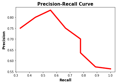
In the above lines of code, we create a plot_pr_curve method which helps us plot the precisions and recalls list on a 2D graph with precision on the x-axis and recall on the y-axis. Notice how the precision starts to drop as recall increases after 0.6.

We have our precision-recall curve, but how do we know at which threshold the model performs the best (i.e., high precision and recall)?

To find out the best precision and recall, we use F1-score to combine precision and recall into a single metric by taking their harmonic mean. A higher F1-score would mean that precision and recall are high, while a lower F1-score signifies a high imbalance between precision and recall (or lower precision and recall).

f1_score = np.divide(2 * (np.array(precisions) * np.array(recalls)), (np.array(precisions) + np.array(recalls)))

print(f1_score)

array([0.71959027, 0.69536849, 0.69536849, 0.69986987, 0.73694181, 0.70606916, 0.70606916, 0.66687977, 0.57106109, 0.46121884])

On Line 1, we compute the f1_score by passing the precisions and recalls list we got from above. From the output, we can observe that the highest f1_score is 0.7369 at index 5.

Now, let’s use the highest f1_score to get the best threshold that balances precision and recall.

precision = precisions[np.argmax(f1_score)]
recall = recalls[np.argmax(f1_score)]
best_threshold = np.round(thresholds[np.argmax(f1_score)], 1)

print(precision, recall, best_threshold)

(0.7, 0.778, 0.4)

From Lines 7-9, we compute the precision, recall, and best threshold by passing the f1_score to the np.argmax function to get the maximum value index in the f1_score array.

Finally, we can conclude that the best threshold to balance precision and recall is 0.4. Another way to put this is to expect our model to achieve optimal precision and recall at the 0.4 threshold.

---

Object Detection Competition Datasets

---

PASCAL VOC 2012

The PASCAL Visual Object Classes 2012 (VOC2012) is a challenge to recognize objects from various visual object classes in a realistic scenario. It is a supervised learning challenge in which the labeled ground-truth images are provided. The dataset has 20 object classes like a person, bird, cat, dog, bicycle, car, chair, sofa, tv, bottle, etc.

The history of PASCAL VOC dates back to the year 2005 when the dataset consisted of only four classes: bicycles, cars, motorbikes, and people. It had a total of 1578 images containing 2209 annotated objects.

Figure 10 shows the sample images from each of the 20 classes, and as we can see, there are several (three) chairs in the second last image in the first row.

The VOC2012 dataset consists of 11,530 images with 27,450 Region of Interest (ROI) annotated objects with a train/val split. The 27,450 ROI refers to the bounding boxes in the entire dataset since each image can have multiple objects or ROI. Hence, there are more than 2X ROIs compared to images.

---

MS COCO

The Microsoft Common Objects in Context (MS COCO) is large-scale object detection, segmentation, and captioning dataset introduced in the year 2014 with the help of extensive crowdsourcing using novel user interfaces. The dataset contains images of 80 object categories with 2.5 million labeled instances in 328k images.

Figure 11 shows the example images from the COCO dataset labeled with instance segmentation.

COCO also has an excellent user interface to explore the images within the dataset. For example, you can select the thumbnails from 80 classes; it will put them in the search bar as tags, and when you search, it will show all the images from the dataset with those tags (classes), as shown in Figure 12.

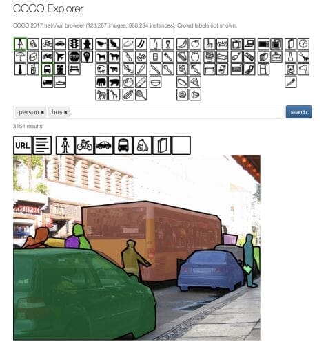
Further, all the classes (more than the searched classes) are displayed as thumbnails when the resulting images are shown. You can play around with it by further clicking on those thumbnails to visualize segmentation masks related to those classes.

---

Precision-Recall Curve for Object Detection

The Precision-Recall curve holds the same or even more importance in evaluating an object detection model’s performance compared to classification. An object detector is considered good if the precision and recall are not impacted when we vary the confidence threshold (probability that a box contains an object). Also, the precision does not decrease as the recall increases.

An ideal object detector with high precision and high recall would have zero false positives (only detect relevant objects) and zero false negatives (not missing relevant objects or predicting all ground-truth objects).

Let’s now try to understand how Precision and Recall curve with the help of an example. For this and subsequent examples, we would use Rafael Padilla’s object detection metrics GitHub repository that provides an excellent summary with examples on precision-recall and average precision.

Consider an example shown in Figure 13; seven images consist of 15 ROIs or ground-truth bounding boxes (shown in green) and 24 ROI proposals or predicted bounding boxes (shown in red). Each of the predicted bounding boxes has a confidence score associated with it.

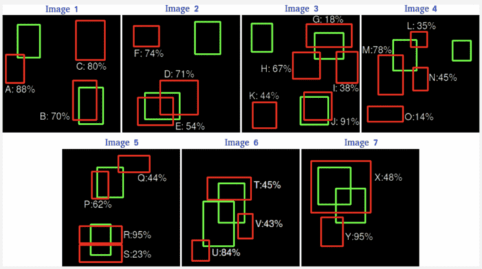
Now let’s transfer all these seven images data into Table 1, which has four columns: image names, detections, a confidence score for each detection, and True Positive (TP) or False Positive (FP). For this example, assume the .

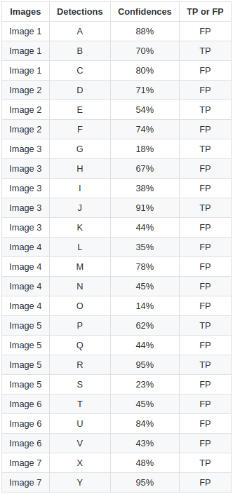
For Image 1, we have three detections: A, B, and C with their respective confidence scores 88%, 70%, and 80% and whether these detections are TP or FP. If we observe Image 1, we can see that the detection A is an FP. This is because it has significantly less overlap with the GT, even though the confidence is high. Remember, we discussed TP/FP in the context of object detection. The detection B seems to be aligned quite well with the GT, so it is marked as a TP, while the detection C is again an FP as there is no GT present for the proposal. And accordingly, we have the TP and FP for the rest of the six images.

We get all TP/FP for the dataset (seven images), but we need to compute TP/FP accumulated over the entire dataset to arrive at the Precision-Recall curve. Therefore, we first arrange the above table rows based on the highest confidence score to the lowest, with which we get a new Table 2.

Table 2 has five more columns: TP/FP are split into two separate columns, accumulated TP, accumulated FP, Precision, and Recall. To calculate Precision and Recall, we use the same formula discussed previously.

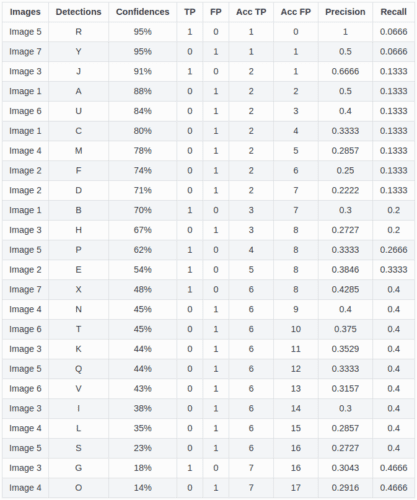
Let’s break down Table 2 into the following steps:

1. We segregate the TP and FP into two columns, and for each proposed ROI, we specify 1 and 0 in their respective columns. For example, in Image 5, detection R is a TP, so we specify 1 in the TP column for the first row, while, in the same image, detection Q is an FP, so we set 1 in the FP column in the 18th row. The same idea is followed for all the proposed ROIs.
2. Once we are through with TP and FP for all the proposed ROIs, we move to the following two columns: Acc TP and Acc FP. Calculating them is pretty simple. For the first row, Acc TP would be the same as TP (i.e., 1). For the second row, it would remain the same as TP is 0. For the third row, it would be 2 as the TP is 1 (so far, two TPs: 1st and 3rd rows). Similarly, we would calculate Acc TP for all the rows until we reach the end.
3. Then, we will follow the same exercise for the Acc FP column and fill all the rows based on the values from the previous Acc FP and current row FP.
4. Now that we have the Acc TP and Acc FP, it is straightforward to calculate the Precision and Recall. For each proposed ROI, we would calculate Precision using the Acc TP and Acc FP, and compute Recall with Acc TP as the numerator and the number of GT as the denominator (TP+FN).
5. For the first row, the Precision will be , which is nothing but 1; for the second row, it will be , which is 0.5, and we will calculate it for all the rows. Similarly, we can calculate the Recall; for example, for the last row, it will be (i.e., 0.466).

Great, now that we have precision and recall values for all the proposed ROIs, we can plot a graph of Precision vs. Recall, as shown in Figure 14.

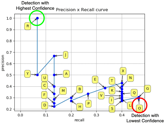
As we can see from the above figure, we have our Precision-Recall curve that shows all the proposed ROIs with the highest confidence score R at the top-left shown in green and the detection with the lowest confidence score displayed at the bottom-right in red color.

Now that we have the Precision-Recall (PR) curve, the next step is to calculate the area under the PR curve (i.e., Average Precision (AP)). However, before calculating the AP, we need to smooth out the zig-zag pattern (i.e., the noise from the above graph) since the precision and recall keep going up and down.

---

Calculating the Average Precision

As learned above, Average Precision (AP) finds the area under the precision-recall curve; we can compute the Average Precision from the PR curve using the 11-point interpolation technique introduced in the PASCAL VOC challenge.

Let’s see how we can apply this technique to the PR curve and arrive at the Average Precision.

---

11-Point Interpolation

The 11-point interpolation calculates the Precision at the Recall levels of (i.e., 11 equally spaced recall levels), and then averages them out. Mathematically it can be expressed as:

where is the measured precision at recall .

Since Precision and Recall are between 0 and 1, the AP also falls between 0 and 1. Therefore, before calculating the AP, we need to smooth out the zig-zag pattern from the PR curve.

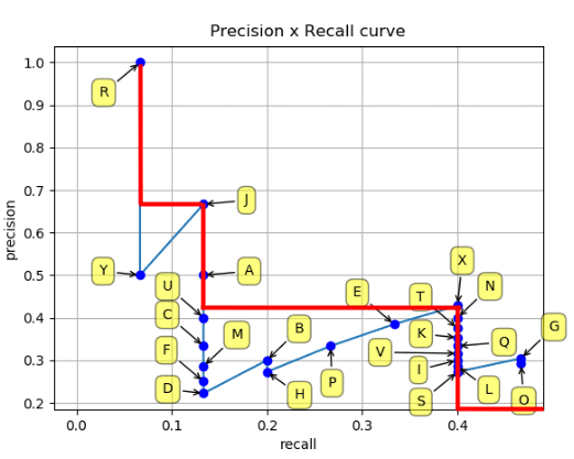
At each recall level, we replace each precision value with the maximum precision value to the right of that recall level, as shown in Figure 16.

So the blue line is transformed into the red lines, and the curve will decrease monotonically instead of the zig-zag pattern. As a result, the calculated AP value will be less susceptible to slight variations in the ranking. Mathematically, we replace the precision value for recall ȓ with the maximum precision for any recall ≥ ȓ.

Once we have this graph, we can divide the recall values from 0 to 1.0 into 11 equal intervals of 0.1 to arrive at Figure 17.

Let’s now compute the AP based on the below 11-point interpolated graph:

Note: According to the original researcher, the intention of interpolating the precision/recall curve is to reduce the impact of the “wiggles” in the precision/recall curve caused by slight variations in the ranking of examples.

---

Mean Average Precision (mAP)

We can calculate the mAP by simply taking the mean over all the class APs. For example, in the PASCAL VOC dataset, we can compute an AP for each of the 20 categories and then average over all the 20 AP classes to get the mean average precision.

Table 3 shows the mAP of various detectors (e.g., SSD300 and SSD512) on the PASCAL VOC dataset and AP of each of the 20 classes. The AP over each class gives a more fine-grained evaluation of the object detector since it tells about the classes where the detector did well and the classes in which the detector performed poorly.

---

Evaluating the YOLOv4 Model Using the COCO Evaluator

This final section will learn to evaluate the object detection model’s performance using the COCO evaluator. We will use the YOLOv4 object detector trained on the MS COCO dataset, and it achieved state-of-the-art results: 43.5% AP (65.7% AP50) for the MS COCO dataset at a real-time speed of ∼65 FPS on the Tesla Volta100 GPU.

We would evaluate the YOLOv4 model on the 2017 MS COCO Validation dataset with 5000 images of varying sizes with the ground truth in COCO format.

---

COCO mAP Evaluator

The COCO evaluator is now the gold standard for computing the mAP of an object detector. Most of the research papers provide benchmarks for the COCO dataset using the COCO evaluation from the past few years. And there are two main reasons. First, the dataset is much richer than the VOC dataset. Secondly, the COCO evaluation does a much deeper analysis of the detection model, thereby providing complete results.

As learned in PASCAL VOC evaluation, a proposed ROI is considered True Positive if with the ground truth. Since there is only one threshold, hence, a detection that very closely aligns () with the ground truth would be considered similar to the one with .

Having a single IoU threshold to assess our detection model might not be a good idea since a single threshold can induce a bias in the evaluation metric. Also, it can be lenient for the model. Therefore, the COCO mAP evaluator averages the mAP of 80 classes over 10 IoU thresholds from 0.5 to 0.95 with a step size of 0.05 (AP@[0.5:0.05:0.95]).

It is worth noting that, unlike PASCAL VOC, the COCO evaluator uses 101-point interpolated AP (i.e., it calculates the precision values at 101 recall levels [0:0.01:1]).

Figure 18 shows the variation of object detection evaluation that the COCO evaluator provides us with, which we will also learn to calculate in the next section of the tutorial.

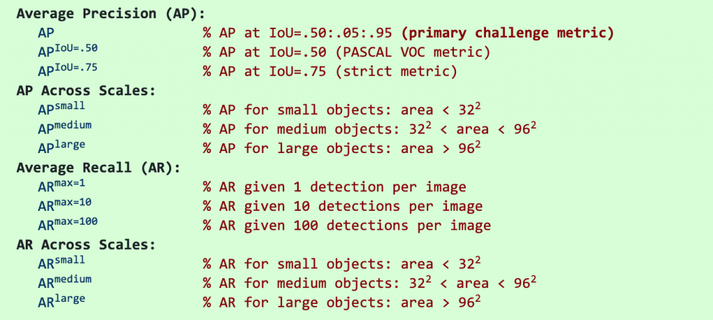
The above figure shows that the COCO evaluator can report AP in various ways, that is, AP@[0.5:0.05:0.95], AP@0.5, AP@0.75, AP across three scales (small, medium, and large).

AP across three scales can be very beneficial if your use case requires you to detect a lot of small objects, then you would want to maximize .

Figure 19 shows the COCO format of the ground truth in the JSON format. It has an optional info field with some information about the year of data publication, version, and URL related to the dataset.

Then, the image field contains the image’s metadata like width, height, file_name, etc.

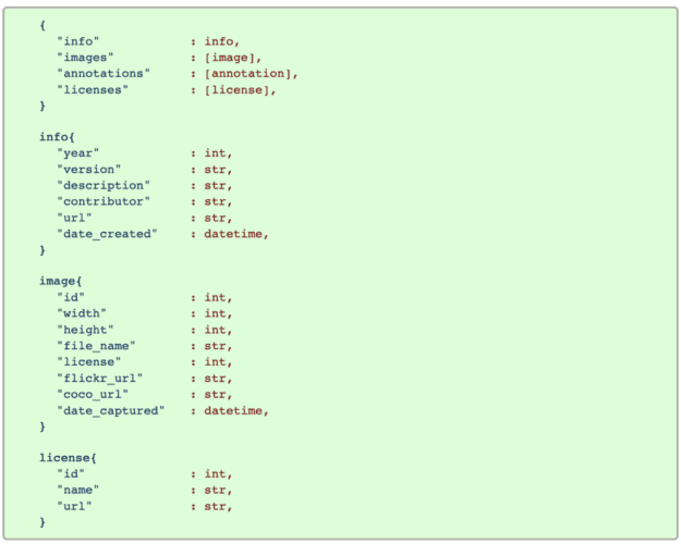
Since the COCO dataset is not just for object detection tasks but also for segmentation, image captioning, and keypoint detection, the annotations would differ for each task. Let’s see what the annotations format looks like for object detection.

Figure 20 shows the object detection annotation and categories fields. The annotation field has image_id, which would be the same for all ROIs, category_id that is the class id, area would be the area of the bounding box (), bbox – top-left corner coordinates, width, and height of the bounding box.

Finally, the categories field will have class data (i.e., class id, class name (car, person)) and supercategory. So, for example, a car and bicycle would have the same supercategory (i.e., vehicle).

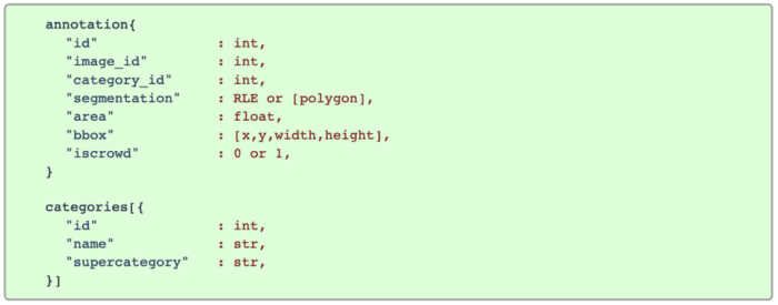
But we do not have to convert our dataset ground-truth to the above COCO format since the COCO Val2017 dataset is already in the desired format.

This was about the ground-truth format, but let’s see how the prediction format in COCO looks.

As we can see in Figure 21, the prediction format is quite simple; we have the image_id: image name, category_id: class id, bbox: top-left coordinates, width and height of bounding box, and score: confidence score of predictions.

Now that we fully understand the ground-truth and prediction COCO format, let’s get straight into the code and compute the mean average precision of the YOLOv4 model.

Note: We will use YOLOv4 from AlexeyAB’s Darknet Repository, and configuring it in Google Colab is a cakewalk.

---

Configuring the Prerequisites

For today’s task, we will use the MS COCO Val 2017 dataset. We created this dataset for object detection, segmentation, and image captioning purposes. It contains 5000 images in the validation set.

Before proceeding to the code, be sure you have configured the Darknet framework and downloaded the YOLOv4 weights and the MSCOCO Val 2017 images and labels.

If you are using a non-Linux system, you can get the dataset here. This will initiate the zipped dataset’s download. Then, extract the contents of this zip file to the project’s data directory.

If you are using a Linux system, you can simply follow the instructions below:

$ cd data
$ wget http://images.cocodataset.org/zips/val2017.zip
$ unzip val2017.zip
$ wget -c http://images.cocodataset.org/annotations/annotations_trainval2017.zip
$ unzip annotations_trainval2017.zip
$ wget https://github.com/AlexeyAB/darknet/releases/download/yolov4/yolov4.weights
$ cd ../

On Line 1, we first change the directory to data, then on Lines 2 and 3, we download and unzip the val2017 images. Then, we download and unzip the ground-truth annotations on Lines 4 and 5. Finally, on Line 6, we download the YOLOv4 weights file.

To compute mean average precision, we open the utils_map.py script, which has a few very important methods for detecting objects: converting bounding boxes to the required format, loading pickle files, running inference over the image directory, and finally storing them prediction in JSON format.

# import the necessary packages
from pyimagesearch import config
from progressbar import progressbar
from darknet import darknet
import pickle
import json
import cv2
import os

def image_detection(imagePath, network, classNames, thresh):
	# image_detection takes the image as an input and returns
	# the detections to the calling function
	width = darknet.network_width(network)
	height = darknet.network_height(network)
	
	# create an empty darknetImage of shape [608, 608, 3]
	darknetImage = darknet.make_image(width, height, 3)

	# read the image from imagePath, convert from BGR->RGB
	# resize the image as per YOLOv4 network input size
	image = cv2.imread(imagePath)
	imageRGB = cv2.cvtColor(image, cv2.COLOR_BGR2RGB)
	imageResized = cv2.resize(imageRGB, (width, height),
		interpolation=cv2.INTER_LINEAR)

	darknet.copy_image_from_bytes(darknetImage, imageResized.tobytes())
	
	# detections include the class labels, bounding box coordinates, and
	# confidence score for all the proposed ROIs in the image
	detections = darknet.detect_image(network, classNames, darknetImage,
		thresh=thresh)
	darknet.free_image(darknetImage)
	
	# return the detections and image shape to the calling function
	return (detections, image.shape)

The first method we define is image_detection. As the name suggests, it takes the image as an input and returns the detections to the calling function (Lines 10-35).

The detections include the class labels, bounding box coordinates, and confidence score for all the proposed ROIs in the image. We also return the raw image shape since we would need this later to scale the predicted bounding box coordinates.

From Lines 13-17, we define the network input width and height which it gets from the yolov4.cfg file and create an empty darknetImage of shape [608, 608, 3].

Then from Line 21-24, we read the image from the path, convert the image to RGB color space since OpenCV reads in BGR format and resize the image as per the network width and height.

Next, we copy the contents of the image to the empty darknetImage and finally call the detect_image method with a few parameters like the network, classNames, darknetImage, and thresh. It then returns detections with proposed bounding box coordinates, class labels, and a confidence score for each proposed ROI.

Finally, we return the detections and image.shape to the calling function on Line 35.

def bbox2points(bbox, img_shape):
    #from bounding box yolo format centerx, centery, w, h
    #to corner points top-left and bottom right
    (x, y, w, h) = bbox

    # compute scale ratio dividing by 608
    hRatio = img_shape[0] / config.YOLO_NETWORK_HEIGHT
    wRatio = img_shape[1] / config.YOLO_NETWORK_WIDTH
    xMin = int(round(x - (w / 2)))
    yMin = int(round(y - (h / 2)))

    # scale them as per the original image size
    return (xMin * wRatio, yMin * hRatio, w * wRatio, h * hRatio)

From Lines 37-49, we define the bbox2points method that accepts bbox coordinates and img_shape: the shape of the input image fed to the model.

The YOLOv4 model outputs the bounding box predictions in format where and are the center coordinates of the bounding box, and are the width and height of the bounding box. These coordinates are normalized per network input size (i.e., 608) since we use the YOLOv4 model with 608 input resolution.

However, we need to convert the bounding box predictions into format and also scale them as per the original image size. We do this so that the bbox prediction format matches the ground-truth bbox format.

We compute the scale ratio on Lines 43 and 44 by dividing the original image size by the network input size . Then we calculate the top-left coordinates: xmin and ymin and finally return the scaled top-left, width, and height of the bounding box to the calling function.

def load_yolo_cls_idx(path):
    # load pickle files: COCO 'class_id' to the
    # class_name list and the COCO 0-90 class ids list
    with open(path, "rb") as f:
        out = pickle.load(f)
        return out

The load_yolo_cls_idx function is a utility function that loads the COCO class_id to the class_name list and the COCO 0-90 class ids list. We need to map the COCO 0-80 class ids to 0-90 class ids since the COCO Val2017 ground-truth category_id ranges from 0 to 90.

def run_inference(imagePaths, network, class_names,
    label2idx, yolo_cls_90, conf_thresh, pred_file):
    results = []

    # loop over all the images
    for path in progressbar(imagePaths):
        # pass the imagePath, network, class names and confidence
        # threshold to image_detection method that returns detections
        # and original image shape
        detections, imgShape = image_detection(
            path, network, class_names, thresh=conf_thresh
        )

       # extract imageID
       imageId = int(os.path.splitext(os.path.basename(path))[0])

       # loop over all the proposed ROIs
       for cls, conf, box in detections:
           (x, y, w, h) = bbox2points(box, imgShape)
           label = [key for key, value in label2idx.items()
                   if value == cls][0]
           label = yolo_cls_90[label]

           # append result for each ROI as per COCO prediction
           # in a dictionary format
           results.append({"image_id": imageId,
                           "category_id": label,
                           "bbox": [x, y, w, h],
                           "score": float(conf)})

           # save the results on disk in a JSON format
           with open(pred_file, "w") as f:
               json.dump(results, f, indent=4)

The run_inference method is where most of the magic happens:

• Iterating over the images to calling image_detection for detections
• Get the imageId from the tail of the path
• Looping over proposed detections
• Transforming the proposed bounding box coordinates with the bbox2points method
• Then extracting label id and converting them to 0-90 class index
• Appending all the required information in a results list
• Finally, creating and dumping the results in a JSON format

Now that most of the work is done in our previous script, we define the eval_map.py script, which is the main driver script that loads the YOLOv4 model from the disk and calls the required methods in the utils_map.py script. Finally, it uses the COCOeval APIs to compute the mAP of the YOLOv4 detector on the COCO Val 2017 dataset.

# import the necessary packages
from pyimagesearch.utils_map import run_inference
from pyimagesearch.utils_map import load_yolo_cls_idx
from pyimagesearch import config
from pycocotools.cocoeval import COCOeval
from pycocotools.coco import COCO
from darknet import darknet

def compute_map():
	# use the COCO class to load and read the ground-truth annotations
	cocoAnnotation = COCO(annotation_file=config.COCO_GT_ANNOTATION)
	
	# call the darknet.load_network method, which loads the YOLOv4
	# network based on the configuration, weights, and data file
	(network, classNames, _) = darknet.load_network(
			config.YOLO_CONFIG,
			config.COCO_DATA,
			config.YOLO_WEIGHTS,
		)

	label2Idx = load_yolo_cls_idx(config.LABEL2IDX)
	yoloCls90 = load_yolo_cls_idx(config.YOLO_90CLASS_MAP)

	# call the run_inference function to generate prediction JSON file
	run_inference(config.IMAGES_PATH, network, classNames, label2Idx,
		yoloCls90, config.CONF_THRESHOLD, config.COCO_VAL_PRED)	

On Line 11, we use the COCO class to load and read the ground-truth annotations.

From Lines 15-19, we call the darknet.load_network method, which loads the YOLOv4 network based on the configuration, weights, and data file. For example, if the configuration file has width and height set to 512, it will create the model accordingly. It also returns us the class names.

We then load the label2Idx dictionary and yoloCls90 map list on Lines 21 and 22.

Now that we have the image_paths list defined, a network created, class names, and other helper files loaded, we can call the run_inference function on Lines 25 and 26 by passing these as parameters. Once the function execution is complete, a COCO_Val_Prediction.json file is created, and the sample prediction JSON is shown in Figure 22.

	# load detection JSON file from the disk
	cocovalPrediction = cocoAnnotation.loadRes(config.COCO_VAL_PRED)

	# initialize the COCOeval object by passing the coco object with
	# ground truth annotations, coco object with detection results
	cocoEval = COCOeval(cocoAnnotation, cocovalPrediction, "bbox")
	
	# run evaluation for each image, accumulates per image results
	# display the summary metrics of the evaluation
	cocoEval.evaluate()
	cocoEval.accumulate()
	cocoEval.summarize()

On Line 29, we load the prediction annotation file that is generated by the run_inference() method.

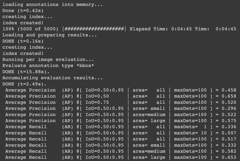
Then, on Line 33, we initialize the COCOeval object by passing the coco object with ground-truth annotations (instances_val2017.json) and the coco object with detection results (COCO_Val_Predictions.json). The third parameter is interesting; it is the IoUType which can be segm for segmentation evaluation, keypoints for keypoint detection evaluation. However, we need to evaluate an object detection model, so we pass bbox.

Finally, from Lines 37-39, we call three functions sequentially:

• cocoEval.evaluate which runs evaluation for each image
• cocoEval.accumulate that accumulates per image results
• cocoEval.summarize that displays the summary metrics of the evaluation

Finally comes the moment of truth! The YOLOv4 model achieved 65.8mAP@0.5 IoU and 45.8mAP@[0.5:0.95] Average IoU on the COCO Val 2017 dataset (Figure 23). It took a total of 267 seconds for the run_inference method to complete, which means the YOLOv4 model achieved more than 19 FPS on a Tesla T4; however, this number could vary on Google Colab.

---

---

Summary

Congratulations on making it this far! We hope you learned a lot through this tutorial, so let’s summarize what we learned quickly.

1. We started by discussing the concept of IoU, why we use IoU, and learned to compute IoU in Python.
2. Then we discussed Precision and Recall from a classification perspective, which helped us understand True Positives, False Positives, and False Negatives from an object detection context with examples.
3. Next, we discussed two of the most popular object detection datasets, PASCAL VOC and MS COCO, which also devised ways to compute mAP with 11-point and 101-point interpolation.
4. We then discussed the Precision-Recall curve for object detection and learned to calculate the Average Precision using the 11-point interpolation technique with the help of an example.
5. Finally, we learned how to evaluate the YOLOv4 model on the MS COCO Val2017 dataset with a COCO evaluator in Python.

---

Citation Information

Sharma, A. “Mean Average Precision (mAP) Using the COCO Evaluator,” PyImageSearch, D. Chakraborty, P. Chugh, A. R. Gosthipaty, S. Huot, K. Kidriavsteva, R. Raha, and A. Thanki, eds., 2022, https://pyimg.co/nwoka

@incollection{Sharma_2022_mAP,
  author = {Aditya Sharma},
  title = {Mean Average Precision {(mAP)} Using the {COCO} Evaluator},
  booktitle = {PyImageSearch},
  editor = {Devjyoti Chakraborty and Puneet Chugh and Aritra Roy Gosthipaty and Susan Huot and Kseniia Kidriavsteva and Ritwik Raha and Abhishek Thanki},
  year = {2022},
  note = {https://pyimg.co/nwoka},
}

---

To download the source code to this post (and be notified when future tutorials are published here on PyImageSearch), simply enter your email address in the form below!