Table of Contents
- Achieving Optimal Speed and Accuracy in Object Detection (YOLOv4)
- Configuring Your Development Environment
- Having Problems Configuring Your Development Environment?
- Introduction to YOLOv4
- Components in an Object Detector
- Bag of Freebies (BoF)
- Bag of Specials (BoS)
- YOLOv4 Architecture Selection
- Selection of BoF and BoS
- CutMix Data Augmentation (Backbone → BoF)
- Mosaic Data Augmentation (Backbone → BoF)
- Class Label Smoothing (Backbone → BoF)
- Self-Adversarial Training (Detector → BoF)
- CSP: Cross-Stage Partial Connection (Backbone → BoS)
- Modified SPP: Spatial Pyramid Pooling (Detector → BoS)
- Path Aggregation Network (Detector → BoS)
- Spatial Attention Module (Detector → BoS)
- DropBlock Regularization (Backbone → BoF)
- Quantitative Benchmarks
- Influence of BoF and Mish Activation on the Backbone
- Influence of BoF on the Detector
- Influence of BoS on the Detector
- Influence of Backbone on the Detector
- Configuring the Darknet Framework and Running Inference with Pretrained YOLOv4 COCO Model
- Summary
Achieving Optimal Speed and Accuracy in Object Detection (YOLOv4)
In this tutorial, you will learn all about YOLOv4 from a research perspective as we will dive deeper into the workings of this accurate and fast object detection network. We would build the intuition by comparing this network with the previous work on object detection.

We believe that YOLOv4 results from many experiments and studies that combine various small novel techniques that improve the Convolutional Neural Network accuracy and speed. But the most challenging part is combining these different features that complement each other, thus providing an optimal and accurate object detection model. And that’s what this paper does in the best way!
Bochkovskiy et al. (2020) did extensive experiments across different GPU architectures and showed that YOLOv4 outperformed all the other object detection network architectures in terms of speed and accuracy. And the purpose of this experiment was to motivate people to leverage the YOLOv4 model’s power without thinking much about the type of GPU since it performs the best even on a conventional GPU which makes this paper even more exciting and unique.
This lesson is the 6th part in our 7-part series on YOLO:
- Introduction to the YOLO Family
- Understanding a Real-Time Object Detection Network: You Only Look Once (YOLOv1)
- A Better, Faster, and Stronger Object Detector (YOLOv2)
- Mean Average Precision (mAP) Using the COCO Evaluator
- An Incremental Improvement with Darknet-53 and Multi-Scale Predictions (YOLOv3)
- Achieving Optimal Speed and Accuracy in Object Detection (YOLOv4) (this tutorial)
- Training the YOLOv5 Object Detector on a Custom Dataset
To learn the novel techniques used and various experiments performed to build a practical YOLOv4 object detector that is fast and accurate and run an inference with YOLOv4 for detecting objects in real-time, just keep reading.
Achieving Optimal Speed and Accuracy in Object Detection (YOLOv4)
In this 6th part of the YOLO series, we will first introduce YOLOv4 and discuss the goal and contributions of YOLOv4 and the quantitative benchmarks. Then, we will discuss the different components involved in an object detector.
Then we will discuss “Bag of Freebies” that help improve the training strategy without impacting the inference cost. We will also discuss the post-processing methods and plugin modules called “Bag of Specials” required to improve the detector’s accuracy that only increase the inference cost by a small amount. Finally, we will also discuss the YOLOv4 Architecture Selection strategy: the backbone, neck with additional blocks, and the head.
From there, we will then discuss the “Bag of Freebies” and “Bag of Specials” leveraged by the YOLOv4 model to achieve state-of-the-art accuracy and speed:
- CutMix and Mosaic data augmentation
- Class Label Smoothing
- Self-Adversarial Training
- DropBlock regularization
- Cross-Stage Partial Connection
- Spatial Pyramid Pooling
- Spatial Attention Module
- Path Aggregation Network
We will also discuss the quantitative benchmarks of YOLOv4 influenced by various experimental interactions:
- BoF and Mish Activation on the Backbone
- BoF on the Detector
- BoS on the Detector
- Backbone on the Detector
Finally, we will see YOLOv4 in action by running the inference on both images and a video with the pre-trained model on the Tesla V100 GPU.
Configuring Your Development Environment
To follow this guide, you need to have the Darknet Framework compiled and installed on your system. We will use AlexeyAB’s Darknet Repository for this tutorial.
We cover the step-by-step instructions on how to install the darknet framework on Google Colab. However, if you would like to configure your development environment now, consider heading to the Configuring the Darknet Framework and Running Inference with Pretrained YOLOv4 COCO Model section.
Having Problems Configuring Your Development Environment?
All that said, are you:
- Short on time?
- Learning on your employer’s administratively locked system?
- Wanting to skip the hassle of fighting with the command line, package managers, and virtual environments?
- Ready to run the code right now on your Windows, macOS, or Linux system?
Then join PyImageSearch University today!
Gain access to Jupyter Notebooks for this tutorial and other PyImageSearch guides that are pre-configured to run on Google Colab’s ecosystem right in your web browser! No installation required.
And best of all, these Jupyter Notebooks will run on Windows, macOS, and Linux!
Introduction to YOLOv4
After the release of YOLOv3, the original author of YOLO (Joseph Redmon) stopped further development on YOLO and even retired from the field of Computer Vision because of ethical reasons.
In 2020, Alexey Bochkovskiy et al. (the author of a renowned GitHub Repository: Darknet) published the YOLOv4: Optimal Speed and Accuracy of Object Detection paper on arXiv. The authors made the best use of existing novel techniques and features by combining them in such a fashion that resulted in an object detector that achieves optimal speed and accuracy, outperforming other state-of-the-art object detectors, as shown in Figure 2. We can observe from the below figure that YOLOv4 runs twice faster than EfficientDet with comparable performance, and it improves YOLOv3’s mAP and FPS by 10% and 12%, respectively, on the MS COCO dataset.

In object detection models, we have always seen a tradeoff between accuracy and speed. For example, searching for free car parking space in a mall via a video camera running an object detection model is executed by slow accurate models. In contrast, a pothole detection warning is performed by fast inaccurate models. Hence, it is vital to improve the real-time object detector accuracy for accurate driver alert, stand-alone process management, and human input reduction.
But often, the challenge in developing the real-time object detector is deploying them on conventional GPUs and edge devices. Building a solution that operates on these low-end traditional GPUs allows their mass usage at an affordable price.
We know that the most accurate neural network models don’t operate in real-time and require many GPUs for training with large mini-batch sizes. Unfortunately, this also means that it’s hard to deploy them on edge devices. With YOLOv4, the authors try to address this issue by creating a CNN that operates in real-time on a conventional GPU and for which training requires only one traditional GPU. Thus, anyone with a 1080 Ti or 2080 Ti GPU can train this super fast and accurate object detector. To validate their model, the authors tested YOLOv4 on various GPU architectures.
Convolutional Neural Network (CNN) performance depends a lot on the features we use and combine. For example, some features work only on a specific model, problem statement, and dataset. But features like batch normalization and residual connections apply to most models, tasks, and datasets. Thus, these features can be called universal.
The authors leverage this idea and assume a few universal features, including
- Weighted-Residual-Connections (WRC)
- Cross-Stage-Partial-connections (CSP)
- Cross mini-Batch Normalization (CmBN)
- Self-adversarial-training (SAT)
- Mish-activation
- Mosaic data augmentation
- DropBlock regularization
- CIoU loss
The above features are combined to achieve state-of-the-art results: 43.5% mAP (65.7% mAP50) on the MS COCO dataset at a real-time speed of ∼65 FPS on the Tesla V100 GPU.
The YOLOv4 model combined the above and more features to form the “Bag of Freebies” for improving the training of the model and “Bag-of-Specials” for improving the accuracy of the object detector. We will discuss more on this in detail later.
Components in an Object Detector
The end-to-end architecture of an object detector is generally composed of two parts:
- Backbone
- Head
As we learned in previous YOLO posts, a backbone is used as a feature extractor pre-trained with classification tasks on an ImageNet dataset. Object detectors made to train and test on GPU use a heavier backbone (e.g., VGG, ResNet, DenseNet, and Darknet-19/53), while, for the CPU, a lighter backbone (e.g., SqueezeNet, MobileNet, etc.) is used. There is always a tradeoff between speed and accuracy. The lighter backbones are faster but less accurate than the heavier ones.
A head is used to predict bounding box coordinates and class labels of objects. The head can be further divided into two stages (i.e., one-stage and two-stage object detectors). An excellent example of two-stage detectors could be the RCNN family. The ones that most closely represent the one-stage detectors are the YOLO family, SSD, and RetinaNet.
Figure 3 shows the object detection workflow of the one-stage and two-stage detectors, composed of several components: Input, Backbone, Neck, and Head.
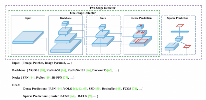
In recent years, object detectors started using a neck, that is, adding a few layers between the backbone and the head for collecting feature maps from different stages of the backbone. For example, in the YOLOv3, the backbone consisted of 53 layers. There were 53 additional layers (including the head) in which features from later layers were upsampled and concatenated with features from early layers.
Generally, a neck is composed of several bottom-up paths, and several top-down paths connect using skip connections. Networks like the Feature Pyramid Network (FPN) and Path Aggregation Network (PAN) work on this mechanism and are often used as a Neck in object detection networks (e.g., YOLOv4 used PANet as the Neck).
Bag of Freebies (BoF)
In almost all cases, an object detector is trained offline, giving the researcher the freedom to develop a training methodology that makes the object detector more accurate without impacting the inference cost. Hence, these methods that only change the training strategy or improve the training cost are known as “bag of freebies” shown in Figure 4.
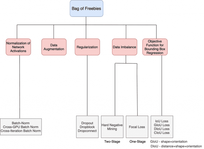
The most common training strategy we use is Data Augmentation, as shown in Figure 5. The purpose of data augmentation is to increase the variability of the input images so that the designed object detection model has higher robustness to the images obtained from different environments.
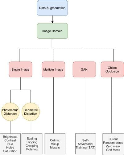
There are various data augmentation categories (e.g., single-image, multiple-image, etc.). As we can see, there are two kinds of distortions in a single image: photometric and geometric. In photometric distortion, you can change the image property by applying brightness, noise, and hue to the image, while, in geometric distortion, we can rotate, crop, or translate the image.
Then some researchers proposed using multiple images together to perform data augmentation like Mixup and CutMix. Mixup uses two images to multiply and superimpose with different coefficient ratios and then adjusts the label with these superimposed ratios. As for CutMix, it covers the cropped image to the rectangle region of other images and adjusts the label according to the size of the mixing area.
YOLOv4 proposed a new multiple image data augmentation technique called Mosaic, which stitches four different images together. More on this in the later section.
Researchers have also proposed Object Occlusion as another data augmentation that has been successful in image classification and object detection. For example, random erase and cutout can randomly select the rectangle region in an image and fill in a random or value of zero. This helps the network from overfitting; for example, given an image of a cat, the network would be forced to learn other parts of its body and classify it as a cat since the cutout would randomly remove its head or tail.
Bag of Specials (BoS)
The “Bag of Specials” are the post-processing methods and plugin modules that only increase the inference cost by a small amount but can significantly improve the accuracy of object detection are called “Bag of Specials.” These modules and methods have a computational load but help boost the accuracy.
These plugin modules are for enhancing specific attributes in a model, such as using Spatial Pyramid Pooling (SPP) for enlarging receptive field, introducing attention mechanism with Spatial Attention Module (SAM), or strengthening feature integration capability with FPN or PAN, etc., and post-processing methods like non-maximum suppression for screening model prediction results.
As shown in Figure 6, we can have numerous choices for each plugin module and the post-processing method. The below figure should be an excellent reference for you when designing your object detection network or training from scratch on your dataset. In YOLOv4, the authors use modified PAN for the feature integration, modified Spatial Attention Module (SAM) as an attention module, and SPP for expanding the receptive field. As for the post-processing method, DIoU-NMS is used in the detector.

In the coming section, we will discuss which modules and methods are employed for training the backbone and the detector. We will also discuss those particular methods in detail.
YOLOv4 Architecture Selection
The main aim is to build a fast operating speed neural network for production systems. To develop such a model, the objective is to find the optimal balance among the
- Input network resolution
- Number of convolution layers
- Number of parameters in the network
- Number of output layers (filters)
The above four points make a lot of sense, keeping in mind that we want to build a reasonably low-cost deployment model. For example, the input network resolution (image size) is essential; the bigger the image size, the more contextual information it has, helping the network easily detect even smaller objects. But the downside of larger image size is that you would need more memory bandwidth, especially on GPU, more network computation (FLOPs), and maybe design a deeper network. Hence, striking a balance between these parameters is essential to building a fast and optimal network.
Backbone
YOLOv4 uses the CSPDarknet53 model as the backbone. Recall that YOLOv3 used the Darknet53 model, and like Darknet53, the CSPDarknet53 is based on DenseNet. Now, what is this CSP prefix in front of it? CSP stands for Cross-Stage Partial connections. We will look into CSP in a later section.
As per previous studies, the CSPResNeXt50 model is considerably better than the CSPDarknet53 model on the image classification task benchmarked on the ImageNet dataset. However, the CSPDarknet53 model is better compared to CSPResNext50 in terms of detecting objects on the MS COCO dataset.
Table 1 shows the network information comparison of CSPDarknet53 with other backbone architectures on the image classification task with the exact input network resolution. We can observe that CSPDarknet53 is the fastest on the RTX 2070 GPU.

The EfficientNet-B3 has the largest receptive field but has the lowest FPS, while the CSPDarknet53 is the fastest with a decent receptive field. Based on the numerous experiments performed, the CSPDarknet53 neural network is the optimal model of the two as the backbone for the detector.
Neck with Additional Block
Next, we need to select the additional blocks for increasing the receptive field and the best method of parameter aggregation from different backbone levels for different detector levels (multi-scale). The choices we have for parameter aggregation are FPN, PAN, ASFF, and BiFPN.
As the receptive field size increases, we get more contextual information around the object and within the image. The authors summarize the role of receptive field size very well in the paper, which is as follows:
- Up to the object size: allows viewing the entire object
- Up to network size: allows viewing the context around the object
- Exceeding the network size: increases the number of connections between the image point and the final activation
To learn more about receptive fields, we recommend you refer to this article by Adaloglou (2020).
Hence, to build a sound detector, you need:
- Higher input network resolution for detecting multiple small-sized objects
- More layers for larger receptive fields to cover the increased size of the input network
- And more parameters for greater capacity of a model to detect multiple objects of different sizes in a single image
Final Architecture
The final architecture YOLOv4 uses CSPDarknet53 backbone, SPP additional module, PANet path-aggregation neck, and YOLOv3 (anchor-based) head, as shown in the high-level overview in Figure 7.

Selection of BoF and BoS
So far, we have discussed the selection of backbone architecture and additional blocks with the neck structure and the head. In this section, we will discuss the choice of BoF and BoS leveraged by YOLOv4. Figures 8 and 9 show the list of BoF and BoS for the backbone and detector. Since there are so many modules and methods used in YOLOv4, we will discuss a few.


CutMix Data Augmentation (Backbone → BoF)
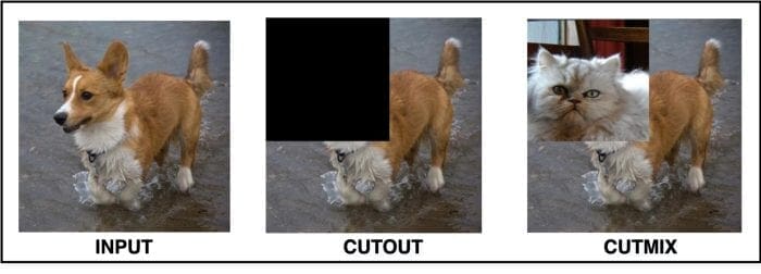
CutMix works similar to the ‘Cutout’ method of image augmentation, rather than cropping a part of the image and replacing it with 0 values. Instead, the CutMix method replaces it with part of a different image.
Cutouts of the image force the model to make predictions based on a robust number of features. Without cutouts, the model relies specifically on a dog’s head to make a prediction. That is problematic if we want to accurately recognize a dog whose head is hidden (perhaps behind a bush). Table 2 shows the results of Mixup, Cutout, and CutMix on ImageNet classification, ImageNet localization, and Pascal VOC 07 detection (transfer learning with SSD finetuning) tasks.

In CutMix, the cutout is replaced with a part of another image along with the second image’s ground truth labeling. The ratio of each image is set in the image generation process (e.g., 0.4/0.6). Figure 10 shows the difference between the cutout and CutMix augmentation.
Mosaic Data Augmentation (Backbone → BoF)
The idea of Mosaic data augmentation was taken from Glenn Jocher’s YOLOv3 PyTorch GitHub repository. Mosaic augmentation stitches four training images into one image in specific ratios (instead of only two in CutMix). The benefit of using mosaic data augmentations is
- The network sees more context information within one image and even outside their normal context.
- Allows the model to learn how to identify objects at a smaller scale than usual.
- Batch normalization would have a 4x reduction because it will calculate activation statistics for four different images at each layer. This would reduce the need for a large mini-batch size during training.
We recommend you watch this video to dive deeper into Mosaic data augmentation.
Figure 11 demonstrates a few images with Mosaic data augmentation, and we can see that now each image has so much context compared to a single image. So, for example, in a single image, we have a train, a bicycle, a bike, a boat, etc.

Class Label Smoothing (Backbone → BoF)
Class label smoothing is a regularization technique used in a multi-class classification problem in which class labels are modified. Generally, for a problem statement involving three classes: cat, dog, elephant, the correct classification for a bounding box would represent a one-hot vector of classes [0,0,1], and the loss function is calculated based on this representation.
However, rough labeling would force the model to reach positive infinity for that last element one and negative infinity for the zeros. This would make the model overfit the training data as it would learn to become super good and be overly sure with a prediction close to 1.0. Still, in reality, it is often wrong, overfit, and overlooks the complexities of other predictions somehow.
Following this intuition, it is more reasonable to encode the class label representation to value that uncertainty to some degree. Naturally, the authors choose 0.9, so [0,0,0.9] to represent the correct class. And now, the model’s goal is not to be 100% accurate in predicting the class cat. The same could be applied to the classes that are zero and can be modified to 0.05/0.1.
Self-Adversarial Training (Detector → BoF)
It is well known that the neural network tends to perform poorly even when there is a minimum perturbation in the input image. For example, given a cat image as input with minimum perturbation, the network could classify it as a traffic light even if both the images look visually the same, as shown in Figure 12. The human vision is unaffected by the perturbation, but a neural network suffers from this attack, and you need to force the network to learn that both the images are the same.

The self-adversarial training is done in two forward and backward stages. In the first stage, it performs a forward pass on a training sample. Generally, we adjust the model weights in the backpropagation to improve the model in detecting objects in this image. But here, it goes in the reverse direction like gradient ascent. As a result, it perturbs the image such that it can degrade the detector performance the most. It creates an adversarial attack targeted at the current model even though the new image may look visually similar. In the second stage, the model is trained with this new perturbed image with the original boundary box and class label. This helps create a robust model that generalizes well and reduces overfitting.
CSP: Cross-Stage Partial Connection (Backbone → BoS)
Cross-Stage Partial connection is used in the Darknet53 backbone. In 2016, Gao Huang et al. proposed DenseNet, and as learned earlier, the Darknet53 is based on DenseNet architecture but with a modification (i.e., cross-stage partial connection).
Before we understand the CSP part of the backbone, let’s quickly understand what a DenseNet is?
A DenseNet comprises many dense blocks. Each Dense Block (shown in Figure 13) contains multiple convolution layers, with each layer composed of batch normalization, ReLU, and followed by convolution. Instead of using the output of the last layer only,
takes the output of all previous layers as well as the original as its input (i.e.,
). Each
below outputs four feature maps. Therefore, at each layer, the number of feature maps is increased by four (the growth rate
). As each layer is connected with every other layer in a dense block, the authors believed this improved the gradient flow.

By stacking multiple such dense blocks, a DenseNet can be formed. As we see in Figure 13, there is a transition layer at the end of the block. This transition layer helps transition from one dense block to another. It is composed of a convolution layer and pooling layer, as shown in Figure 14.

Coming to the CSP part of Darknet53, the original DenseNet has duplicate gradient flow information and is also more computationally expensive. The YOLOv4 authors were inspired by the CSPNet paper that showed that adding cross-stage partial connections to ResNet, ResNext, and DenseNet reduced computation cost and memory usage of these networks and benefited the inference speed and accuracy.
CSPNet separates the input feature maps or the base layer of the DenseBlock into two parts. The first part bypasses the DenseBlock and goes directly as an input to the transition layer. The second part goes through the Dense block, as shown in Figure 15.

Figure 16 shows a more detailed view of the dense block. The convolutional layer is applied to the input feature map, and the convolutional output is concatenated with the input, followed throughout the dense block sequentially. However, the CSP takes only the partial part of the input feature map into the dense block, and the remaining directly goes as an input to the transition layer. This new design reduces the computational complexity by separating the input into two parts, with only one going through the Dense Block.

Modified SPP: Spatial Pyramid Pooling (Detector → BoS)
He et al. (2015) proposed Spatial Pyramid Pooling; the idea was to have multi-scale input image training. The existing convolutional neural networks require a fixed size input image because of the fully connected layer in which you need to specify the fixed input size.
Let’s say your network has many convolutional and max-pooling layers, a fully connected layer. The input to the fully connected layer would be a flattened 1-dimensional vector. If the input to the network keeps varying, then the flattened 1-dimensional vector size would also change, which would result in an error since a fully connected layer expects a fixed size input. The same problem would arise in object detection when the region of interest would be of variable sizes. And that’s where the SPP layer is helpful.
The SPP layer (see Figure 17) helps detect objects of different scales. It replaces the last pooling layer with a spatial pyramid pooling layer. First, the feature maps are spatially divided into bins with
, say, equals 1, 2, and 4. Then a maximum pool is applied to each bin for each channel. This forms a fixed-length representation that can be further analyzed with fully connected layers. This solves the problem because now you can pass arbitrary size input to the SPP layer, and the output would always be a fixed-length representation.
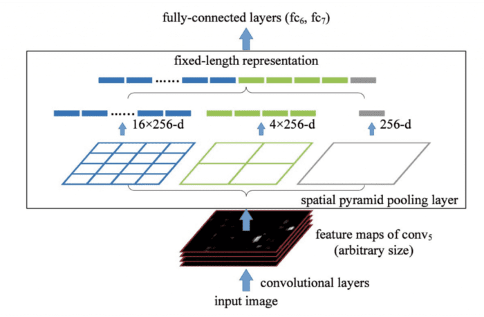
In YOLO, the SPP is modified to retain the output spatial dimension. A spatial pyramid pooling block with three max-pooling layers is shown in Figure 18. The SPP layer is added after the last convolutional layer in CSPDarknet53. The feature maps are pooled in different scales; the maximum pool is applied to a sliding kernel of size, say, ,
,
,
. The spatial dimension is preserved, unlike traditional SPP, where the feature maps are resized into feature vectors with a fixed size.

The features maps from different kernel sizes are then concatenated along with the input feature maps of the SPP block to get the output feature maps. This way we get feature maps that extract and converge the multi-scale local region features as the output for object detection.
The authors claim that the modified SPP has a larger receptive field which benefits the detector.
Path Aggregation Network (Detector → BoS)
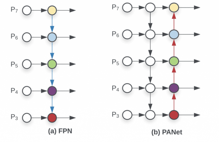
PANet is used for the Neck of the model. PAN is an improvement over the Feature Pyramid Network. PAN adds a bottom-up pathway on top of the FPN (shown in Figure 19(b)) and is used to ensure that the most useful information is used from each feature level. In FPN, information is combined from neighboring layers in the bottom-up and top-down stream.
Figure 19 shows PAN for object detection. A bottom-up path (b) is added to make the low-layer information flow easily to the top. In FPN, the localized spatial information traveled upward, shown with the red arrow. While not clearly demonstrated in the diagram, the red path goes through about 100+ layers. PAN introduced a short-cut path (the green path) which only takes about 10 layers to go to the top layer. These short-circuit concepts make fine-grain localized information available to top layers.

In FPN, objects are detected separately and independently at different scale levels. This, according to the PANet authors, may produce duplicated predictions and not utilize information from other scale feature maps. Instead, PAN fuses the data from all layers, as shown in Figure 19 (c). To learn more about this, please refer to the paper.
The side-by-side comparison between FPN and PANet is shown in Figure 20.
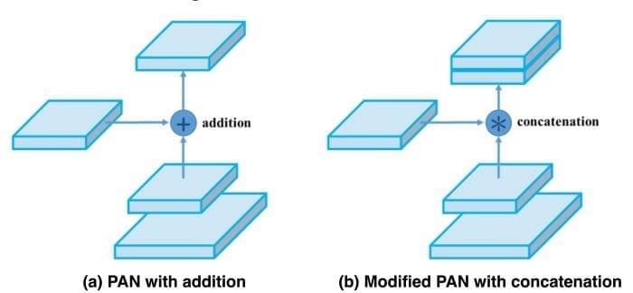
The YOLOv4 authors slightly modified the PAN; instead of adding neighbor layers together, they changed the shortcut connections to the concatenation (Figure 21).
Spatial Attention Module (Detector → BoS)
The spatial attention module comes from the work published by Woo et al. (2018) on Convolutional Block Attention Module (CBAM), shown in Figure 22. The idea of this paper was that given an intermediate feature map, the module sequentially infers attention maps along two separate dimensions, channel and spatial. Both attention maps masks were multiplied by the input feature map to output refined feature maps.

But going back to the history of attention models, even before CBAM in 2017, the Squeeze and Excitation (SE) Network was introduced, a channel-wise attention model. The SE allowed the network to perform feature recalibration by suppressing the less useful information and emphasizing informative features. The squeezing part would apply average pooling over the feature maps resulting in a vector output, and the excitation part was a multi-layer perceptron. Finally, the excitation output was multiplied by the input feature maps to get refined features.
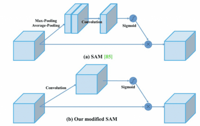
YOLOv4 uses only the Spatial Attention Module (SAM) from the CBAM shown in Figure 23 because the GPU’s channel-wise attention module is inefficient. In SAM, a max pool and average pool are applied separately to input feature maps along the channel to create two sets of feature maps.

Then, all the input channels are squeezed into one channel, and the max pool and average pool outputs are concatenated. The concatenated results are fed into a convolution layer followed by a sigmoid function to create a spatial attention mask. To get the final output, an element-wise multiplication is performed using spatial attention.
In YOLOv4, the SAM is modified from spatial-wise attention to point-wise attention. In addition, the maximum and average pooling layers are replaced with a convolution layer, as shown in Figure 24.
DropBlock Regularization (Backbone → BoF)
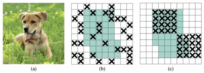
The DropBlock regularization technique is similar to the Dropout regularization used to prevent overfitting. However, in Dropout block regularization, the dropped feature points are no longer spread randomly but are combined into blocks, and the entire block is dropped. As shown in Figure 25(b), dropping out of activations at random is ineffective in removing semantic information because nearby activations contain closely related information. Instead, dropping continuous regions can remove certain semantic information (e.g., head or feet) (shown in Figure 25(c)) and consequently enforce remaining units to learn features for classifying input images.
Quantitative Benchmarks
The authors pretrained the backbone with the classification task on the ImageNet dataset and the detector for the object detection task on the MS COCO 2017 dataset.
Influence of BoF and Mish Activation on the Backbone
The influence of BoF and Activation function on the CSPResNeXt-50 classifier is shown in Table 3. From the table, it is evident that the authors did an ablation study. Based on the study and experiment performed, the authors found that with CutMix, Mosaic, Label Smoothing, and Mish activation function (last row in Table 3), the CSPResNeXt-50 classifier performed the best. It achieved 79.8% Top-1 accuracy and 95.2% Top-5 accuracy.
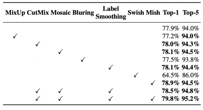
The authors performed similar experiments with the CSPDarknet-53 backbone. They found that with the same setting (i.e., CutMix, Mosaic, Label Smoothing, and Mish), they achieved a 78.7% Top-1 accuracy and 94.8% Top-5 accuracy (shown in Table 4).

Based on the above experiments, the authors concluded that CSPResNeXt-50 outperformed the CSPDarknet-53 in the classification task.
Influence of BoF on the Detector
The further study concerns the influence of different Bag-of-Freebies on the detector training accuracy, as shown in Table 5. From this table, it is evident that with grid sensitivity, mosaic augmentation, IoU threshold, genetic algorithm, and GIoU/CIoU loss, the CSPResNeXt50-PANet-SPP detector achieves the best mean average precision. Also, changing the loss from GIoU to CIoU has zero effect on the detection accuracy.

Influence of BoS on the Detector
By adding the Spatial Attention Module to the CSPResNeXt50-PANet-SPP as a Bag-of-Specials along with PANet and SPP, we can see an improvement in the mean average precision of the detector in Table 6.

Influence of Backbone on the Detector
This is exciting as we compare the two backbones with the detector: the CSPResNeXt-50 and the CSPDarknet-53. We learned earlier from Tables 3 and 4 that CSPResNeXt-50 outperformed the CSPDarknet-53 on the image classification task.
However, when we use these two backbones with the detector, we can see from Table 7 that CSPDarknet53-PANet-SPP is the clear winner in terms of mean average precision and average precision with 0.5 and 0.75 IoU. Hence, the conclusion is that the Darknet-53 is suitable for the detection task, so the authors chose Darknet as the detector.

Configuring the Darknet Framework and Running Inference with Pretrained YOLOv4 COCO Model
In our previous posts on YOLOv1, YOLOv2, and YOLOv3, we learned to configure the darknet framework and ran inference with the pre-trained YOLO models; we would follow the same steps as before configuring the darknet framework. Then, finally, run the inference with the YOLOv4 pre-trained model and compare the results with previous YOLO versions.
Configuring the darknet framework and running the inference with YOLOv4 on images and video is divided into seven easy-to-follow steps. So, let’s get started!
Note: Please be sure you have the matching CUDA, CUDNN, and NVIDIA Driver Installed on your machine. For this experiment, we use CUDA-10.2 and CUDNN-8.0.3. But if you plan to run this experiment on Google Colab, do not worry, as all these libraries come pre-installed with it.
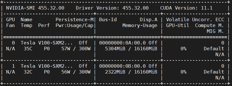
Step #1: We will use the GPU for this experiment, so make sure the GPU is up and running with the following command:
# Sanity check for GPU as runtime
$ nvidia-smi
Figure 26 shows the GPUs available in the machine (i.e., V100), driver, and CUDA versions.
Step #2: We will install a few libraries like OpenCV, FFmpeg, etc., that would be required before compiling and installing darknet.
# Install OpenCV, ffmpeg modules
$ apt install libopencv-dev python-opencv ffmpeg
Step #3: Next, we clone the modified version of the darknet framework from the AlexyAB repository. As learned earlier, Darknet is an open-source neural network written by Joseph Redmon. It is written in C and CUDA, supporting both CPU and GPU computation. However, unlike in previous YOLO versions, this time, the creator of YOLOv4 is AlexyAB itself.
# Clone AlexeyAB darknet repository
$ git clone https://github.com/AlexeyAB/darknet/
$ cd darknet/
Be sure to change the directory to darknet since, in the next step, we will configure the Makefile and compile it. Also, do a sanity check using !pwd; we should be in the /content/darknet directory.
Step #4: Using stream editor (sed), we will edit the make files and enable flags: GPU, CUDNN, OPENCV, and LIBSO.
Figure 27 shows a snippet of the Makefile, the contents of which are discussed later:

- We enable the
GPU=1andCUDNN=1to build darknet withCUDAto perform and accelerate the inference on theGPU. NoteCUDAshould be in/usr/local/cuda; otherwise, the compilation will result in an error but don’t worry if you compile it on Google Colab. - If your
GPUhas Tensor Cores, enableCUDNN_HALF=1to gain up to3Xinference and2Xtraining speedup. Since we use a Tesla V100 GPU that has tensor cores, we will enable this flag. - We enable
OPENCV=1to build darknet withOpenCV. This will allow us to detect video files, IP cameras, and other OpenCV off-the-shelf functionalities like reading, writing, and drawing bounding boxes over the frames. - Finally, we enable
LIBSO=1to build thedarknet.solibrary and a binary runnableuselibfile that uses this library. Enabling this flag allows us to use Python scripts for inference on images and videos, and we will be able to importdarknetinside it.
Now, let’s edit the Makefile and compile it.
# Enable the OpenCV, CUDA, CUDNN, CUDNN_HALF & LIBSO Flags and Compile Darknet
$ sed -i 's/OPENCV=0/OPENCV=1/g' Makefile
$ sed -i 's/GPU=0/GPU=1/g' Makefile
$ sed -i 's/CUDNN=0/CUDNN=1/g' Makefile
$ sed -i 's/CUDNN_HALF=0/CUDNN_HALF=1/g' Makefile
$ sed -i 's/LIBSO=0/LIBSO=1/g' Makefile
$ make
The make command will take around 90 seconds to finish the execution. Now that the compilation is complete, we are all set to download the YOLOv4 weights and run the inference.
Step #4: We will now download the YOLOv4 COCO weights. Since Alexey Bochkovskiy is the primary author of YOLOv4, the weights of this model are available on his Darknet GitHub repository and can be downloaded from here. There are various configurations and weight files available (e.g., YOLOv4, YOLOv4-Leaky, and YOLOv4-SAM-Leaky). We will download the original YOLOv4 model weights with input resolution .
# Download YOLOv4 Weights
$ wget https://github.com/AlexeyAB/darknet/releases/download/
darknet_yolo_v3_optimal/yolov4.weights
Step #5: Now, we will run the darknet_images.py script to infer the images.
# Run the darknet image inference script
$ python3 darknet_images.py --input data --weights \
yolov4.weights --config_file cfg/yolov4.cfg \
--dont_show
Let’s put some light on the command line arguments we pass to darknet_images.py:
--input: Path to the images directory or text file with the path to the images or a single image name. Supportsjpg,jpeg, andpngimage formats. In this case, we pass the path to the image folder calleddata.--weights: YOLOv4 weights path.--config_file: Configuration file path of YOLOv4. On an abstract level, this file stores the neural network model architecture and a few other parameters (e.g.,batch_size,classes,input_size, etc.). We recommend you give a quick read of this file by opening it in a text editor.--dont_show: This will disable OpenCV from displaying the inference results, and we use this since we are working with Google Colab.
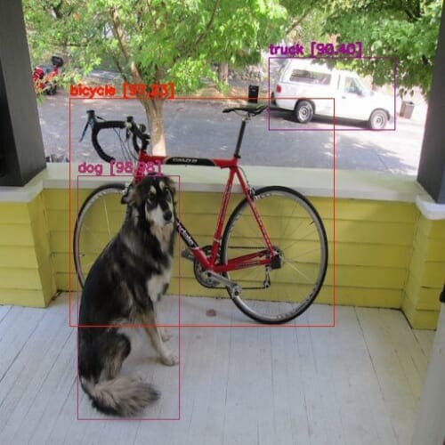
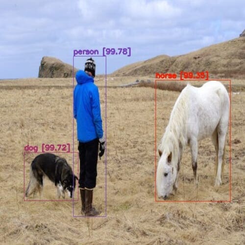
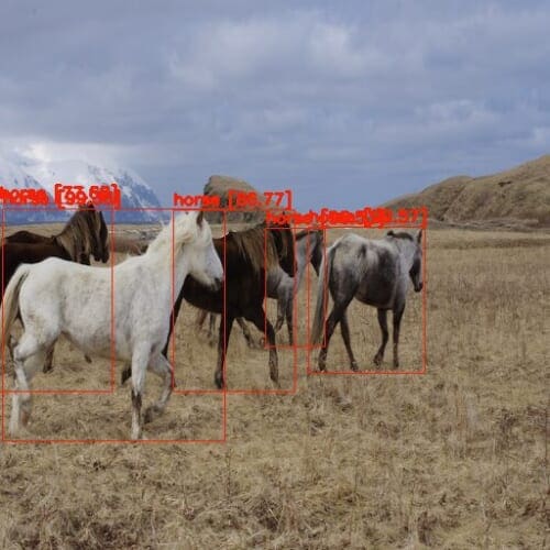
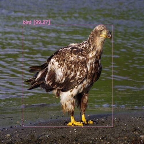
After running the YOLOv4 pre-trained COCO model on the below images, we learn that the model makes zero mistakes and perfectly detects the objects in all the images. Compared to YOLOv3, which missed one horse, YOLOv4 detects all five horses. In addition, we observed confidence score improvement in YOLOv3; we see a similar trend in YOLOv4 since it detects objects with even more confidence than YOLOv3.
We can see from Figure 28 that the model correctly predicts a dog, bicycle, and truck with a very high confidence score.
In Figure 29, the model detects all three objects correctly with almost 100% confidence, quite similar to the YOLOv3 network.
Recall that YOLOv3 missed detecting one horse, but the YOLOv4 model didn’t leave any room for error and did excellently well by detecting all the horses correctly and with very high confidence (Figure 30). This was a bit of a complex image to crack as it has a group of overlapping horses. Still, we all can take a moment to appreciate how the YOLO versions evolved, becoming better both in accuracy and speed.
Finally, in Figure 31, a much easier one that all the variants could detect, the YOLOv4 model also detects it correctly.
Step #6: Now, we will run the pre-trained YOLOv4 model on a small clip from the movie Skyfall.
Before running the darknet_video.py demo script, we will first download the video from YouTube using the pytube library and crop the video with the moviepy library. So let’s quickly install these modules and download the video.
# Install pytube and moviepy for downloading and cropping the video
$ pip install git+https://github.com/rishabh3354/pytube@master
$ pip install moviepy
# Import the necessary packages
$ from pytube import YouTube
$ from moviepy.video.io.ffmpeg_tools import ffmpeg_extract_subclip

# Download the video in 720p and Extract a subclip
$ YouTube('https://www.youtube.com/watch?v=tHRLX8jRjq8'). \ streams.filter(res="720p").first().download()
$ ffmpeg_extract_subclip("/content/darknet/Skyfall.mp4", \
0, 30, targetname="/content/darknet/Skyfall-Sample.mp4")
Step #7: Finally, we will run the darknet_video.py script to generate predictions for the Skyfall video. We print the FPS information over each frame of the output video.
Be sure to change the video codec in the set_saved_video function from MJPG to mp4v at Line 57 in darknet_video.py if using an mp4 video file; otherwise, you will get a decoding error while playing the inference video.
# Change the VideoWriter Codec
fourcc = cv2.VideoWriter_fourcc(*"mp4v")
Now that all the necessary installations and modifications are complete, we will run the darknet_video.py script:
# Run the darknet video inference script
$ python darknet_video.py --input \
/content/darknet/Skyfall-Sample.mp4 \
--weights yolov4.weights --config_file \
cfg/yolov4.cfg --dont_show --out_filename \
pred-skyfall.mp4
Let’s look at the command line arguments we pass to darknet_video.py:
--input: Path to the video file or 0 if using a webcam--weights: YOLOv4 weights path--config_file: Configuration file path of YOLOv4--dont_show: This will disable OpenCV from displaying the inference results--out_filename: Inference results output video name, if empty, the output video is not saved.
Below are the inference results on the Skyfall Action Scene Video. The detection is dense and, without a doubt, the best out of all the YOLO variants. The YOLOv4 network achieves an average of 81 FPS on the Tesla V100 GPU with mixed-precision (83 FPS reported by the author).
What's next? We recommend PyImageSearch University.
86+ total classes • 115+ hours hours of on-demand code walkthrough videos • Last updated: April 2026
★★★★★ 4.84 (128 Ratings) • 16,000+ Students Enrolled
I strongly believe that if you had the right teacher you could master computer vision and deep learning.
Do you think learning computer vision and deep learning has to be time-consuming, overwhelming, and complicated? Or has to involve complex mathematics and equations? Or requires a degree in computer science?
That’s not the case.
All you need to master computer vision and deep learning is for someone to explain things to you in simple, intuitive terms. And that’s exactly what I do. My mission is to change education and how complex Artificial Intelligence topics are taught.
If you're serious about learning computer vision, your next stop should be PyImageSearch University, the most comprehensive computer vision, deep learning, and OpenCV course online today. Here you’ll learn how to successfully and confidently apply computer vision to your work, research, and projects. Join me in computer vision mastery.
Inside PyImageSearch University you'll find:
- ✓ 86+ courses on essential computer vision, deep learning, and OpenCV topics
- ✓ 86 Certificates of Completion
- ✓ 115+ hours hours of on-demand video
- ✓ Brand new courses released regularly, ensuring you can keep up with state-of-the-art techniques
- ✓ Pre-configured Jupyter Notebooks in Google Colab
- ✓ Run all code examples in your web browser — works on Windows, macOS, and Linux (no dev environment configuration required!)
- ✓ Access to centralized code repos for all 540+ tutorials on PyImageSearch
- ✓ Easy one-click downloads for code, datasets, pre-trained models, etc.
- ✓ Access on mobile, laptop, desktop, etc.
Summary
Congratulations on making it this far! YOLOv4 is a very long topic, and we know it was a lot to digest as we discussed everything in detail, so let’s quickly summarize:
- We started by introducing YOLOv4 and discussing the authors’ contributions to designing a fast and accurate object detector. We touched upon the speed and accuracy benchmark comparisons between YOLOv4 and state-of-the-art detectors. We also learned the different components involved in an object detector.
- You were then introduced to “Bag of Freebies,” what they are composed of, and their role in improving the training strategy without impacting the inference cost.
- You then learned the post-processing methods and plugin modules called “Bag of Specials,” which improve the detector’s accuracy with minimal effect on the inference speed.
- We then discussed how YOLOv4 Architecture was selected: the backbone it used, the Neck with additional blocks, and the YOLOv2 head for object detection.
- You then learned the “Bag of Freebies” used by the YOLOv4 model (e.g., cutmix, mosaic, class label smoothing, self-adversarial training, and dropblock regularization).
- We then discussed the “Bag of Specials” leveraged by the YOLOv4 model (e.g., CSP, SPP, SAM, and PAN).
- Then we discussed the quantitative benchmarks of YOLOv4. We discussed the Influence of BoF and Mish Activation on the Backbone, Influence of BoF on the Detector, Influence of BoS on the Detector, and Influence of Backbone on the Detector.
- Finally, we ran the Inference with the pretrained YOLOv4-COCO model on images and video on a Tesla V100 and compared the detection results with earlier YOLO models.
We have almost reached the end of this series; by learning YOLOv4, you are very close to mastering the YOLO family. We hope you enjoyed learning about the YOLO detection models and would use the concepts learned in this tutorial to devise a model of your own.
Citation Information
Sharma, A. “Achieving Optimal Speed and Accuracy in Object Detection (YOLOv4),” PyImageSearch, D. Chakraborty, P. Chugh, A. R. Gosthipaty, S. Huot, K. Kidriavsteva, R. Raha, and A. Thanki, eds., 2022, https://pyimg.co/c6kiu
@incollection{Sharma_2022_YOLOv4,
  author = {Aditya Sharma},
  title = {Achieving Optimal Speed and Accuracy in Object Detection ({YOLOv4})},
  booktitle = {PyImageSearch},  editor = {Devjyoti Chakraborty and Puneet Chugh and Aritra Roy Gosthipaty and Susan Huot and Kseniia Kidriavsteva and Ritwik Raha and Abhishek Thanki},
  year = {2022},
  note = {https://pyimg.co/c6kiu},
}

Join the PyImageSearch Newsletter and Grab My FREE 17-page Resource Guide PDF
Enter your email address below to join the PyImageSearch Newsletter and download my FREE 17-page Resource Guide PDF on Computer Vision, OpenCV, and Deep Learning.


Comment section
Hey, Adrian Rosebrock here, author and creator of PyImageSearch. While I love hearing from readers, a couple years ago I made the tough decision to no longer offer 1:1 help over blog post comments.
At the time I was receiving 200+ emails per day and another 100+ blog post comments. I simply did not have the time to moderate and respond to them all, and the sheer volume of requests was taking a toll on me.
Instead, my goal is to do the most good for the computer vision, deep learning, and OpenCV community at large by focusing my time on authoring high-quality blog posts, tutorials, and books/courses.
If you need help learning computer vision and deep learning, I suggest you refer to my full catalog of books and courses — they have helped tens of thousands of developers, students, and researchers just like yourself learn Computer Vision, Deep Learning, and OpenCV.
Click here to browse my full catalog.