Table of Contents
- An Incremental Improvement with Darknet-53 and Multi-Scale Predictions (YOLOv3)
- Configuring Your Development Environment
- Having Problems Configuring Your Development Environment?
- Introduction to YOLOv3
- What Is YOLO?
- Darknet-53 Network Architecture
- Class Prediction
- Quantitative Results
- Configuring the Darknet Framework and Running Inference with the Pretrained YOLOv3 COCO Model
- Summary
An Incremental Improvement with Darknet-53 and Multi-Scale Predictions (YOLOv3)
In this tutorial, you will learn the improvements made in YOLOv2; more specifically, we will look at the design changes that significantly improved the performance of YOLO, giving rise to a new version of YOLO called YOLOv3. The significant difference between YOLOv3 and its predecessors is in the network architecture called Darknet-53, which we will explore in detail in the coming section of the tutorial. We will also demonstrate using the YOLOv3 model pretrained on the 80 class MS COCO dataset.
YOLOv3 was one of the best models in terms of real-time object detection in 2019.
If you followed along with the previous tutorials on YOLO, then understanding this would not be a challenge since there aren’t many modifications, and most concepts are acquired from YOLOv1 and YOLOv2.
This lesson is the 5th of our 7-part series on YOLO:
- Introduction to YOLO Family
- Understanding a Real-Time Object Detection Network: You Only Look Once (YOLOv1)
- A Better, Faster, and Stronger Object Detector (YOLOv2)
- Mean Average Precision (mAP) Using the COCO Evaluator
- An Incremental Improvement with Darknet-53 and Multi-Scale Predictions (YOLOv3) (this tutorial)
- Achieving Optimal Speed and Accuracy in Object Detection (YOLOv4)
- Training the YOLOv5 Object Detector on a Custom Dataset
To learn the network architecture modifications made to the YOLOv3 object detector and see a demo of detecting objects in real-time, just keep reading.
An Incremental Improvement with Darknet-53 and Multi-Scale Predictions (YOLOv3)
In this 5th part of the YOLO series, we will start by introducing YOLOv3. Then, we will briefly revisit the YOLO object detection general concept.
From there, we will discuss the new Darknet-53 architecture of YOLOv3 in detail, covering:
- Pretraining stage
- Detection stage
- Prediction across three scales
- Network’s output prediction tensor
- Feature extraction
- Use of anchor boxes
- Modification in the loss function: Class prediction with sigmoid
We would discuss the quantitative benchmarks comparing YOLOv3 with Faster-RCNN, YOLOv2, SSD, and RetinaNet.
Finally, we will put YOLOv3 into practical use by installing the Darknet framework and running the inference on images and video with the MS COCO pretrained model on the Tesla V100 GPU.
Configuring Your Development Environment
To follow this guide, you need to have the Darknet Framework compiled and installed on your system. We will use AlexeyAB’s Darknet Repository for this tutorial.
We cover the step-by-step instructions on installing the Darknet framework on Google Colab. However, if you would like to configure your development environment now, consider heading to the Configuring the Darknet Framework and Running Inference with the Pretrained YOLOv3 COCO Model section.
Having Problems Configuring Your Development Environment?
All that said, are you:
- Short on time?
- Learning on your employer’s administratively locked system?
- Wanting to skip the hassle of fighting with the command line, package managers, and virtual environments?
- Ready to run the code right now on your Windows, macOS, or Linux system?
Then join PyImageSearch University today!
Gain access to Jupyter Notebooks for this tutorial and other PyImageSearch guides that are pre-configured to run on Google Colab’s ecosystem right in your web browser! No installation required.
And best of all, these Jupyter Notebooks will run on Windows, macOS, and Linux!
Introduction to YOLOv3
Following the YOLOv2 paper, In 2018, Joseph Redmon (a Graduate Student at the University of Washington) and Ali Farhadi (an Associate Professor at the University of Washington) published the YOLOv3: An Incremental Improvement paper on arXiv. The authors made many design changes concerning the network architecture, adapting most of the other techniques from the previous YOLO versions.
The YOLOv3 paper introduced a new network architecture called Darknet-53 as opposed to the Darknet-19 architecture in YOLOv2. The Darknet-53 is a more extensive network than before but is much more accurate and faster. It is trained at various image resolutions as seen in YOLOv2; at resolution, YOLOv3 achieves 28.2 mAP runs at 45 FPS and is as accurate as Single-Shot Detector (SSD321) but 3x faster (Figure 2). The authors performed the quantitative benchmarks on the Titan X GPU.
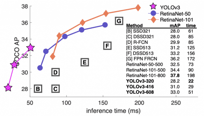
 -axis (Redmon and Farhadi (2018), p. 1, fig. 1).
Unlike before, in YOLOv3, the authors compare the mAP at various IOUs; at 0.5 IOU, it achieves 57.9 in 51ms compared to 57.5
in 198 ms by RetinaNet-101-800. Thus, though both achieve almost the same mAP, YOLOv3 is 3.8x faster than RetinaNet.
What Is YOLO?
YOLO stands for “You Only Look Once.” It is a single-stage object detector that leverages the power of convolutional neural networks to detect multiple objects in a given image. It divides the image into a grid and predicts class probabilities and box coordinates for each grid cell of the image.
YOLO applies a single neural network on the whole image and detects the objects in a single network pass. This architecture is similar in spirit to an image classification network where the object is classified in a single forward pass. Thus, YOLO is faster than other state-of-the-art detectors, making it ideal for many industrial applications.
Darknet-53 Network Architecture
Table 1 shows the Darknet-53 architecture consisting of 53 convolutional layers that act as a base for the object detection network or a feature extractor. The 53 layers are pretrained on the image classification task using the ImageNet dataset. For the object detection task, 53 more layers are stacked on top of the base/backbone network, making it a total of 106 layers, and we get the final model known as YOLOv3.
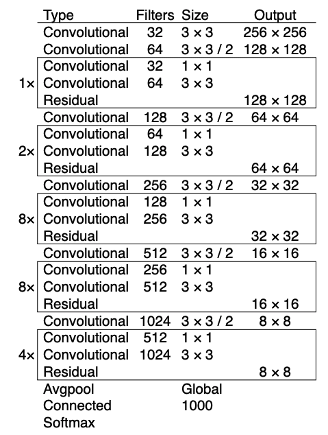
In YOLOv2, the authors used a much smaller network consisting of 19 layers; however, as the deep learning field progressed, we were introduced to much wider and deeper networks such as ResNet, DenseNet, etc. Inspired by new classification networks, YOLOv3 was deeper than its predecessor and borrowed ideas like residual blocks (skip connection with addition) and skip connection with concatenation to avoid vanishing gradient problems and help propagate information that helped predict objects at different scales.
The important parts to note in YOLOv3 network architecture are residual blocks, skip connections, and upsampling layers.
Darknet-53 network architecture is more potent than Darknet-19 and more efficient than ResNet-101 and ResNet-152. As shown in Table 2, Darknet-53 performs more billion floating-point operations per second than other backbone architectures, making it efficient. This also means the network structure better utilizes the GPU, making it more efficient to evaluate and thus faster. Furthermore, in terms of Top-1 and Top-5 image classification accuracy, Darknet-53 performs better than Darknet-19 and performs similar to ResNet. The below results are benchmarked on the ImageNet dataset, and inference is computed on a Titan X GPU.

Pretraining Stage
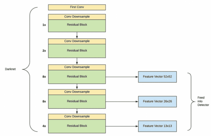
The Darknet-53 architecture was trained on the image classification task with the ImageNet dataset in the pretraining step. The architecture is simple and self-explanatory, but let’s look at some of the main components. After every convolutional layer, a residual group (shown with a rectangle) has varying residual blocks such as 1x, 2x, 4x, and 8x. To downsample the spatial dimension of the feature maps, strided convolution with a stride of 2 is used before every residual group. This helped prevent the loss of low-level features and encode positional information useful for object detection; moreover, since strided convolution has parameters, the downsampling would not be entirely non-parametric as max-pooling. It improved the ability to detect smaller objects.
The number of filters starts with 32 and is doubled at every convolutional layer and a residual group. Each residual block has a bottleneck structure filter followed by a
filter followed by a residual skip connection. Finally, for image classification in the last layers, we have a fully connected layer and a softmax function for outputting a 1000 class probability score.
Detection Stage
In the detection step, the layers after the last residual group are removed (i.e., the classification head), giving us the backbone for our detector. Since YOLOv3 is supposed to detect objects at multiple scales at each of the last three residual groups, a detection layer is attached to make object detection predictions, as shown in Figure 3. The figure below shows that the output from the three residual groups is extracted as a feature vector at three different scales and fed into the Detector. Assuming the input to the network is , the three feature vectors we obtain are
,
, and
, responsible for detecting small, medium, and large objects, respectively.
Prediction Across Three Scales
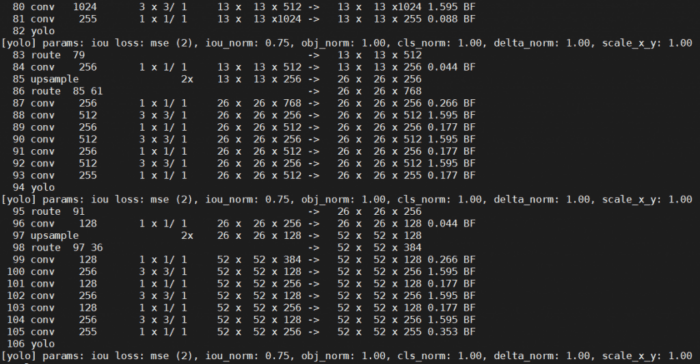
In previous YOLO architectures, the detection occurred only at the final layer; however, in YOLOv3, the objects are detected at three different stages/layers of the network, namely 82, 94, and 106 (Figure 4).
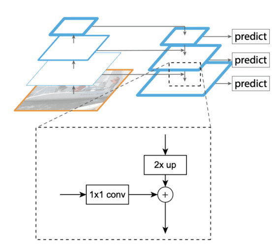
The network extracts features from each of the three scales using a similar concept to feature pyramid networks or FPN. We will not detail what feature pyramid networks are, but in short, the structure of FPN has a bottom-up pathway, top-down pathway, and lateral connections (Figure 5). The idea behind using FPN is to improve ConvNet’s pyramidal feature hierarchy having varying level semantics and build feature pyramids with high-level semantics throughout. And the goal is to combine low-resolution features (in later layers of the network), which are very informative, with high-resolution features (in initial layers of the network). Thus, FPN helps improve the problem of recognizing objects that are at vastly different scales.
From Figure 6, we can see that several convolutional layers are added on top of the base feature extractor. The last layer for each scale predicts a 3D tensor encoding: bounding box coordinates, objectness score, and class predictions. For the COCO dataset, three bounding boxes are predicted at each scale (three-box priors/anchors for each scale). So the output prediction tensor is for the four bounding box offsets, one objectness score prediction, and 80 class predictions. For detecting medium-scale objects, large-scale features are upsampled and concatenated. Similarly, for detecting small-scale objects, medium-scale features are upsampled and concatenated. This setting allowed small-scale detection to benefit from both medium and large detections.
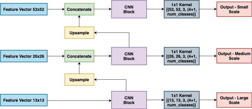
Upsampling and concatenating features with different scales allows the network to learn more fine-grained information from the earlier feature maps and more meaningful semantic information from the upsampled later layer feature maps.
Similar to YOLOv2, for choosing the precise priors/anchors, the authors use -means clustering in YOLOv3. But instead of five, in YOLOv3, nine clusters are selected, dividing them evenly across the three scales, which means three anchors for each scale per grid cell.
Class Prediction
Both YOLOv1 and YOLOv2 used sum-squared error for bounding box class prediction instead of commonly used softmax (for multilabel classification). However, in YOLOv3, the class prediction is treated as a multilabel classification problem which means the class labels are treated as mutually non-exclusive. The authors found that using sigmoid or logistic classifiers for predicting class labels for each bounding box was more beneficial than softmax.
During training, binary cross-entropy loss was used for the class predictions. This setting helps when we move to more complex datasets like the Open Images Dataset. This dataset contains many mutually non-exclusive (or overlapping) labels like a Woman and Person; hence, using a softmax imposes the assumption that each box has precisely one class which is often not the case. A multilabel approach better models the data.
Quantitative Results
This section compares YOLOv3 (trained with input resolution) with state-of-the-art two-stage and single-stage object detectors benchmarked on the COCO dataset. As shown in Table 3, YOLOv3 does a decent job in mAP though it’s not the best. The table shows various AP columns; however, in previous YOLO versions, the performance was benchmarked on just AP50 (i.e., at 0.5 IOU). These different AP columns measure the performance of the models in a more fine-grained way; here, AP{50,75} is average precision at 0.5 and 0.75 IOU, AP{s,m,l} means average precision for small, medium, and large objects.
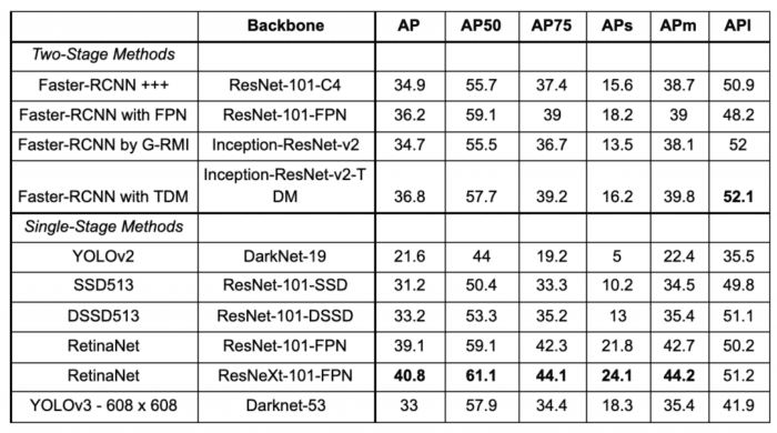
We learned from Figure 2 that YOLOv3 performed on par with SSD variants but was 3x faster. It is still quite far from other models like RetinaNet. When we look at the AP50 results, YOLOv3 does quite well and performs on par with almost all the detectors. But as we increase the IOU threshold to 0.75, the performance drops significantly, indicating that YOLOv3 struggles to get the boxes perfectly aligned with the object. Earlier YOLO versions struggled to detect small objects, but YOLOv3, with its multi-scale training approach, performs relatively well, achieving 18.3 APs. However, it has comparatively worse performance on medium and larger-size objects.
From these results, we can conclude that YOLOv3 performs better at AP50 and is, of course, the fastest among all the other object detectors.
Configuring the Darknet Framework and Running Inference with the Pretrained YOLOv3 COCO Model
In our previous two posts on YOLOv1 and YOLOv2, we learned to configure the Darknet framework and ran inference with the pretrained YOLO models; we would follow the same steps as before configuring the Darknet framework. Then, finally, run the inference with the YOLOv3 pretrained model and see it perform better than its previous versions.
Configuring the Darknet framework and running the inference with YOLOv3 on images and video is divided into eight easy-to-follow steps. So, let’s get started!
Note: Please ensure you have the matching CUDA, CUDNN, and NVIDIA Driver Installed on your machine. For this experiment, we use CUDA-10.2 and CUDNN-8.0.3. But if you plan to run this experiment on Google Colab, do not worry, as all these libraries come pre-installed with it.
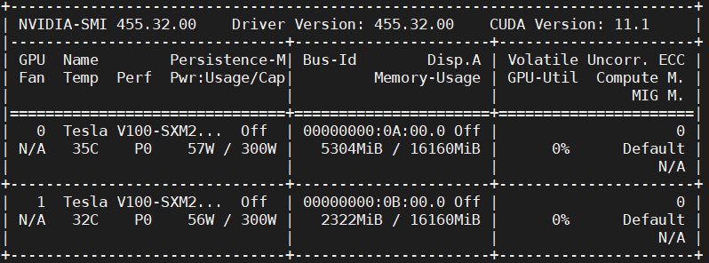
Step #1: We will use the GPU for this experiment to ensure the GPU is up and running.
# Sanity check for GPU as runtime
$ nvidia-smi
Figure 7 shows the GPUs available in the machine (i.e., V100), driver, and CUDA versions.
Step #2: We will install a few libraries like OpenCV, FFmpeg, etc., that would be required before compiling and installing Darknet.
# Install OpenCV, ffmpeg modules
$ apt install libopencv-dev python-opencv ffmpeg
Step #3: Next, we clone the modified version of the Darknet framework from the AlexyAB repository. As learned earlier, Darknet is an open-source neural network written by Joseph Redmon. It is written in C and CUDA, supporting both CPU and GPU computation. The official implementation of the Darknet is available at: https://pjreddie.com/darknet/; we will download the YOLOv3 weights provided by the official website.
# Clone AlexeyAB darknet repository
$ git clone https://github.com/AlexeyAB/darknet/
$ cd darknet/
Be sure to change the directory to darknet since, in the next step, we will configure the Makefile and compile it. Also, do a sanity check using !pwd; we should be in the /content/darknet directory.
Step #4: Using stream editor (sed), we will edit the make files and enable flags: GPU, CUDNN, OPENCV, and LIBSO.
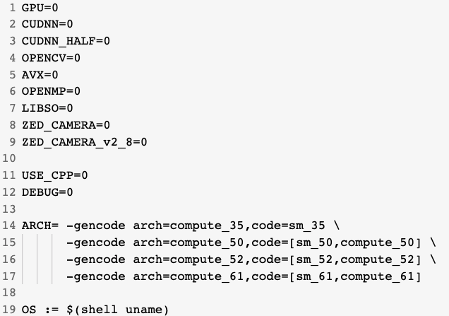
Figure 8 shows a snippet of the Makefile contents, which are discussed later:
- We enable the
GPU=1andCUDNN=1to build darknet withCUDAto perform and accelerate the inference on theGPU. NoteCUDAshould be in/usr/local/cuda; otherwise, the compilation will result in an error, but don’t worry if you are compiling it on Google Colab. - If your
GPUhas Tensor Cores, enableCUDNN_HALF=1to gain up to 3X inference and 2X training speedup. Since we use a Tesla V100 GPU that has tensor cores, we will enable this flag. - We enable
OPENCV=1to build darknet with OpenCV. This will allow us to detect video files, IP cameras, and other OpenCV off-the-shelf functionalities like reading, writing, and drawing bounding boxes over the frames. - Finally, we enable
LIBSO=1to build thedarknet.solibrary and binary runnable fileuselibthat makes use of this library. Enabling this flag would allow us to use Python scripts for inference on images and videos, and we will be able to importdarknetinside it.
Now let’s edit the Makefile and compile it.
# Enable the OpenCV, CUDA, CUDNN, CUDNN_HALF & LIBSO Flags and Compile Darknet
$ sed -i 's/OPENCV=0/OPENCV=1/g' Makefile
$ sed -i 's/GPU=0/GPU=1/g' Makefile
$ sed -i 's/CUDNN=0/CUDNN=1/g' Makefile
$ sed -i 's/CUDNN_HALF=0/CUDNN_HALF=1/g' Makefile
$ sed -i 's/LIBSO=0/LIBSO=1/g' Makefile
$ make
The make command will take around 90 seconds to finish the execution. Now that the compilation is complete, we are all set to download the YOLOv3 weights and run the inference.
Step #5: We will now download the YOLOv3 COCO weights from the official YOLOv3 documentation.
# Download YOLOv3 Weights
$ wget https://pjreddie.com/media/files/yolov3.weights
Step #6: Now, we will run the darknet_images.py script to infer the images.
# Run the darknet image inference script
$ python3 darknet_images.py --input data --weights \
yolov3.weights --config_file cfg/yolov3.cfg \
--dont_show
Let’s put some light on the command line arguments we pass to darknet_images.py:
--input: Path to the images directory or text file with the path to the images or a single image name. Supportsjpg,jpeg, andpngimage formats. In this case, we pass the path to the image folder calleddata.--weights: YOLOv3 weights the path.--config_file: Configuration file path of YOLOv3. On an abstract level, this file stores the neural network model architecture and a few other parameters likebatch_size,classes,input_size, etc. We recommend you quickly read this file by opening it in a text editor.--dont_show: This will disable OpenCV from displaying the inference results, and we use this since we are working with Google Colab.
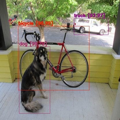
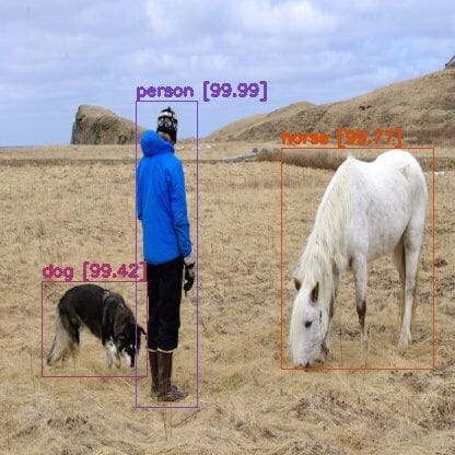
After running the YOLOv3 pretrained MS COCO model on the below images, we learn that the model hardly makes mistakes and perfectly detects the objects in all the images. Furthermore, in contrast to YOLOv1 and YOLOv2, where we saw few False Positives and False Negatives, YOLOv3 outperforms both, and in fact, it detects the object with a very high confidence score.
We can see from Figure 9 that the model correctly predicts a dog, bicycle, and truck with almost 100% high confidence.
In Figure 10, the model detects all three objects correctly again with 100% confidence. If you remember, YOLOv1 detected a horse as a sheep, while YOLOv2 predicted a horse twice as a horse and sheep.
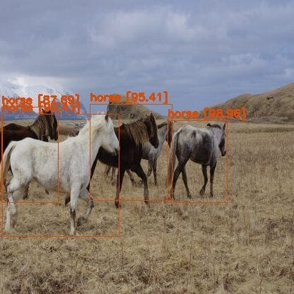
In Figure 11, the model did well by detecting four out of the five horses and with a very high confidence score. However, recall both YOLOv1 and YOLOv2 struggled with this image by either predicting a horse like a cow or failing to detect one of the four horses, and both models predicted them with a very low confidence score.
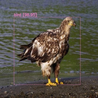
Finally, in Figure 12, the YOLOv3 model predicts an eagle as a bird similar to YOLOv1 and YOLOv2.
Step #7: Now, we will run the pretrained YOLOv3 model on a video from the movie Skyfall; it is the same video that the Authors had used in one of their experiments.
Before running the darknet_video.py demo script, we will first download the video from YouTube using the pytube library and crop the video with the moviepy library. So let’s quickly install these modules and download the video.
# Install pytube and moviepy for downloading and cropping the video
$ pip install git+https://github.com/rishabh3354/pytube@master
$ pip install moviepy
On Lines 2 and 3, we install the pytube and moviepy libraries.
# Import the necessary packages
$ from pytube import YouTube
$ from moviepy.video.io.ffmpeg_tools import ffmpeg_extract_subclip

# Download the video in 720p and Extract a subclip
$ YouTube('https://www.youtube.com/watch?v=tHRLX8jRjq8'). \ streams.filter(res="720p").first().download()
$ ffmpeg_extract_subclip("/content/darknet/Skyfall.mp4", \
0, 30, targetname="/content/darknet/Skyfall-Sample.mp4")
On Lines 2 and 3, we import the pytube and ffmpeg_extract_subclip modules. On Lines 6-8, with the help of the imported modules, we download the Skyfall video from YouTube in 720p resolution. And then, we extract the subclip (first 30 seconds) from the downloaded video using the ffmpeg_extract_subclip module from moviepy.
Step #8: Finally, we will run the darknet_video.py script to generate predictions for the Skyfall video. We print the FPS information over each frame of the output video.
Be sure to change the video codec in the set_saved_video function from MJPG to mp4v at Line 57 in darknet_video.py if using an mp4 video file; otherwise, you will get a decoding error while playing the inference video.
# Change the VideoWriter Codec
fourcc = cv2.VideoWriter_fourcc(*"mp4v")
Now that all the necessary installations and modifications are complete, we will run the darknet_video.py script:
# Run the darknet video inference script
$ python darknet_video.py --input \
/content/darknet/Skyfall-Sample.mp4 \
--weights yolov3.weights --config_file \
cfg/yolov3.cfg --dont_show --out_filename \
pred-skyfall.mp4
Let’s look at the command line arguments we pass to darknet_video.py:
--input: Path to the video file or 0 if using a webcam--weights: YOLOv3 weights path--config_file: Configuration file path of YOLOv3--dont_show: This will disable OpenCV from displaying the inference results--out_filename: Inference results output video name, if empty the output video is not saved.
Below are the inference results on the Skyfall Action Scene Video. The predictions have to be better than YOLOv1 and YOLOv2 since the network learns to predict at multiple scales, reducing the chances of False Negatives. Also, YOLOv3 was trained on the COCO dataset with 80 classes (compared to 20 classes in VOC), so you would see more object categories being detected, like a bottle or tie not present in the VOC dataset. The YOLOv3 network achieves an average of 100 FPS on the Tesla V100 GPU with mixed precision.
What's next? We recommend PyImageSearch University.
86+ total classes • 115+ hours hours of on-demand code walkthrough videos • Last updated: April 2026
★★★★★ 4.84 (128 Ratings) • 16,000+ Students Enrolled
I strongly believe that if you had the right teacher you could master computer vision and deep learning.
Do you think learning computer vision and deep learning has to be time-consuming, overwhelming, and complicated? Or has to involve complex mathematics and equations? Or requires a degree in computer science?
That’s not the case.
All you need to master computer vision and deep learning is for someone to explain things to you in simple, intuitive terms. And that’s exactly what I do. My mission is to change education and how complex Artificial Intelligence topics are taught.
If you're serious about learning computer vision, your next stop should be PyImageSearch University, the most comprehensive computer vision, deep learning, and OpenCV course online today. Here you’ll learn how to successfully and confidently apply computer vision to your work, research, and projects. Join me in computer vision mastery.
Inside PyImageSearch University you'll find:
- ✓ 86+ courses on essential computer vision, deep learning, and OpenCV topics
- ✓ 86 Certificates of Completion
- ✓ 115+ hours hours of on-demand video
- ✓ Brand new courses released regularly, ensuring you can keep up with state-of-the-art techniques
- ✓ Pre-configured Jupyter Notebooks in Google Colab
- ✓ Run all code examples in your web browser — works on Windows, macOS, and Linux (no dev environment configuration required!)
- ✓ Access to centralized code repos for all 540+ tutorials on PyImageSearch
- ✓ Easy one-click downloads for code, datasets, pre-trained models, etc.
- ✓ Access on mobile, laptop, desktop, etc.
Summary
In this tutorial, we introduced an anchor-based YOLOv3 object detection network. We discussed the new Darknet-53 architecture of YOLOv3 in detail, covering:
- Pretraining stage
- Detection stage
- Prediction across three scales
- Network output prediction tensor
- Feature extraction
- Use of anchor boxes
- Modification in the loss function
We ran an Inference with the pretrained YOLOv3 model on images and video on a Tesla V100 and compared the detection results with its predecessors (i.e., YOLOv1 and YOLOv2).
In the next tutorial of our series, you’ll learn about the recent state-of-the-art object detector (YOLOv4) resulting from many experiments and studies that combine various small novel techniques that help achieve Optimal Speed and Accuracy in Object Detection.
Citation Information
Sharma, A. “An Incremental Improvement with Darknet-53 and Multi-Scale Predictions (YOLOv3),” PyImageSearch, D. Chakraborty, P. Chugh, A. R. Gosthipaty, S. Huot, K. Kidriavsteva, R. Raha, and A. Thanki, eds., 2022, https://pyimg.co/8xfpg
@incollection{Sharma_2022_YOLOv3,
  author = {Aditya Sharma},
  title = {An Incremental Improvement with Darknet-53 and Multi-Scale Predictions ({YOLO}v3)},
  booktitle = {PyImageSearch},
  editor = {Devjyoti Chakraborty and Puneet Chugh and Aritra Roy Gosthipaty and Susan Huot and Kseniia Kidriavsteva and Ritwik Raha and Abhishek Thanki},
  year = {2022},
  note = {https://pyimg.co/8xfpg},
}
Unleash the potential of computer vision with Roboflow - Free!
- Step into the realm of the future by signing up or logging into your Roboflow account. Unlock a wealth of innovative dataset libraries and revolutionize your computer vision operations.
- Jumpstart your journey by choosing from our broad array of datasets, or benefit from PyimageSearch’s comprehensive library, crafted to cater to a wide range of requirements.
- Transfer your data to Roboflow in any of the 40+ compatible formats. Leverage cutting-edge model architectures for training, and deploy seamlessly across diverse platforms, including API, NVIDIA, browser, iOS, and beyond. Integrate our platform effortlessly with your applications or your favorite third-party tools.
- Equip yourself with the ability to train a potent computer vision model in a mere afternoon. With a few images, you can import data from any source via API, annotate images using our superior cloud-hosted tool, kickstart model training with a single click, and deploy the model via a hosted API endpoint. Tailor your process by opting for a code-centric approach, leveraging our intuitive, cloud-based UI, or combining both to fit your unique needs.
- Embark on your journey today with absolutely no credit card required. Step into the future with Roboflow.

Join the PyImageSearch Newsletter and Grab My FREE 17-page Resource Guide PDF
Enter your email address below to join the PyImageSearch Newsletter and download my FREE 17-page Resource Guide PDF on Computer Vision, OpenCV, and Deep Learning.


Comment section
Hey, Adrian Rosebrock here, author and creator of PyImageSearch. While I love hearing from readers, a couple years ago I made the tough decision to no longer offer 1:1 help over blog post comments.
At the time I was receiving 200+ emails per day and another 100+ blog post comments. I simply did not have the time to moderate and respond to them all, and the sheer volume of requests was taking a toll on me.
Instead, my goal is to do the most good for the computer vision, deep learning, and OpenCV community at large by focusing my time on authoring high-quality blog posts, tutorials, and books/courses.
If you need help learning computer vision and deep learning, I suggest you refer to my full catalog of books and courses — they have helped tens of thousands of developers, students, and researchers just like yourself learn Computer Vision, Deep Learning, and OpenCV.
Click here to browse my full catalog.