Pixel Shuffle Super Resolution with TensorFlow, Keras, and Deep Learning

When an image is increased in size (spatially, along the width and height), the conventional methods lead to new pixel information getting created which often degrades the image quality giving a soft and blurry image as output. Thankfully, as with most topics in recent years, Deep Learning has given us many viable solutions to tackle this problem.

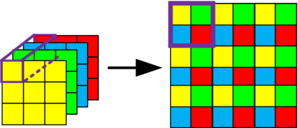
In today’s blog, we will learn how to implement Pixel Shuffle Super Resolution, a beautiful concept that gives us a taste of deep learning’s contributions to the domain of Super Resolution.

This blog will cover:

• Utilizing the BSDS500 dataset
• Understanding the Residual Dense Block architecture
• Implementing Pixel Shuffle
• Showcasing an array of pre- and post-processing methodologies
• Training our own Super-Resolution model
• Drawing inferences from model results
• Assessing the results against standard metrics
• Testing out your own images on the model

By the end of this tutorial, you will have a crystal clear understanding of Pixel Shuffle and the concepts shown here.

You will also be able to define your own Super-Resolution Architecture and have fun with your custom images! If that sounds like fun, let’s jump into it and get started.

To learn how to implement Pixel Shuffle Super Resolution, just keep reading.

Pixel Shuffle Super Resolution with TensorFlow, Keras, and Deep Learning

Recently, NVIDIA had made the news with a creation called Deep Learning Super Sampling (DLSS). It used deep learning to upscale low-resolution images to a higher resolution to fit the display of high-resolution monitors. The catch was that the upscaled image showed quality similar to that of rendering the image natively in a higher resolution.

Along with that, the majority of the computation was done whilst the image was in its lower resolution. This effectively enabled people with weaker computer builds to enjoy games without compromising on the quality. So, how does this happen?

Configuring your development environment

To follow this guide, you need to have the TensorFlow machine learning library installed on your system. For additional image handling purposes, you’ll be using the Python Imaging Library (PIL) and the Imutils library.

Luckily, all the above libraries are pip-installable!

$ pip install tensorflow
$ pip install pillow
$ pip install imutils 

That is all for the environment configuration necessary for this guide!

Having problems configuring your development environment?

All that said, are you:

• Short on time?
• Learning on your employer’s administratively locked system?
• Wanting to skip the hassle of fighting with the command line, package managers, and virtual environments?
• Ready to run the code right now on your Windows, macOS, or Linux system?

Then join PyImageSearch University today!

Gain access to Jupyter Notebooks for this tutorial and other PyImageSearch guides that are pre-configured to run on Google Colab’s ecosystem right in your web browser! No installation required.

And best of all, these Jupyter Notebooks will run on Windows, macOS, and Linux!

Project structure

Before we start implementing Pixel Shuffle Super Resolution, let’s look at the project structure.

Once we have downloaded our project directory, it should look like this:

$ tree .
.
├── generate_super_res.py
├── output
│   ├── super_res_model
│   │   ├── saved_model.pb
│   │   └── variables
│   │       ├── variables.data-00000-of-00001
│   │       └── variables.index
│   ├── training.png
│   └── visualizations
│       ├── 0_viz.png
│       ├── 1_viz.png
│       ├── 2_viz.png
│       ├── 3_viz.png
│       ├── 4_viz.png
│       ├── 5_viz.png
│       ├── 6_viz.png
│       ├── 7_viz.png
│       ├── 8_viz.png
│       └── 9_viz.png
├── pyimagesearch
│   ├── config.py
│   ├── data_utils.py
│   ├── __init__.py
│   └── subpixel_net.py
└── train.py

5 directories, 20 files

The parent directory has two python scripts and two folders.

• generate_super_res.py: This contains the script to use our trained model and generate super-resolution images. It also contains several functions which will be used in pre- and post-processing of the image.
• train.py: The python script will call our defined model, train it, and assess its quality. It also contains custom metric functions we will use for our model.

Next, let’s get into the pyimagesearch directory! In it, we will find 4 python scripts:

• __init__.py: This will make python treat the pyimagesearch directory as a module
• config.py: This script contains various hyperparameter presets and defines the data paths
• data_utils.py: This script will help process the input before it gets fed to our model during training
• subpixel_net.py: This script contains our super-resolution model, which will be called by the train.py script

Lastly, we have the output directory which contains:

• super_res_model: The directory where our trained model will be stored
• training.png: A sample model assessment plot
• visualizations: The directory where all our generated super-resolution images will be stored.

What is Pixel Shuffle Super Resolution?

Super Resolution is an umbrella term for a class of techniques in which accurate or close-to-accurate pixel information is added to construct a high-resolution image from its low-resolution form while maintaining its original quality.

Pixel Shuffle Super Resolution is an upsampling technique where Image Super Resolution is achieved in a rather ingenious method. Feature maps are extracted in its LR (Low-Resolution) space (as opposed to earlier techniques where this was done in the HR (High-Resolution) space).

However, the highlight of this method is a novel efficient sub-pixel convolution layer, which learns an array of filters to upscale the final LR feature maps into the HR output. Not only does this method achieve great success, but it also reduces time complexity, since a chunk of the computation is done while the image is in its low-resolution state.

We also employ the use of Residual Dense Blocks (RDBs), an architecture that heavily focuses on keeping the information extracted in previous layers alive, while computing outputs for the present layer.

Configuring the Prerequisites

For today’s task, we will use the BSDS500, also known as the Berkeley Segmentation Dataset. This dataset was created to specifically help in the field of image segmentation and contains 500 images.

If you are using a non-Linux system, you can get the dataset here (right-click to save link). This will initiate the zipped dataset’s download. Extract the contents of this zip file to the project’s directory.

If you are using a Linux system, you can simply navigate to the project’s directory and execute the following commands:

$ wget http://www.eecs.berkeley.edu/Research/Projects/CS/vision/grouping/BSR/BSR_bsds500.tgz
$ tar xvf BSR_bsds500.tgz

Before diving into the implementation, let’s set up our paths and hyperparameters. For that, we will hop into the module config.py. Most other scripts in our project will call this module and use its presets.

# import the necessary packages
import os

# specify root path to the BSDS500 dataset
ROOT_PATH = os.path.join("BSR", "BSDS500", "data", "images")

# specify paths to the different splits of the dataset
TRAIN_SET = os.path.join(ROOT_PATH, "train")
VAL_SET = os.path.join(ROOT_PATH, "val")
TEST_SET = os.path.join(ROOT_PATH, "test")

First, we will set our ROOT_PATH to the dataset as shown on Line 5. From the ROOT_PATH, we define our training, validation, and test set paths, respectively (Lines 8-10). The BSDS500 is already set up in a way where the dataset is divided into training, validation, and test sets for convenience.

# specify the initial size of the images and downsampling factor
ORIG_SIZE = (300, 300)
DOWN_FACTOR = 3

# specify number of RDB blocks, batch size, number of epochs, and
# initial learning rate to train our model
RDB_LAYERS = 3
BATCH_SIZE = 8
EPOCHS = 100
LR = 1e-3

#define paths to serialize trained model, training history plot, and
# path to our inference visualizations
SUPER_RES_MODEL = os.path.join("output", "super_res_model")
TRAINING_PLOT = os.path.join("output", "training.png")
VISUALIZATION_PATH = os.path.join("output", "visualizations")

Our next job is to set some important hyperparameters:

• ORIG_SIZE: Will be our image’s original and target shape (Line 13)
• DOWN_FACTOR: To determine by what amount we will downsample our original image (Line 14)
• RDB_LAYERS: To specify the number of convolution layers inside a single RDB (Line 18)

Apart from these, we also set the batch size, epochs, and learning rate (Lines 19-21) and define paths to serialize our trained model and history plots (Lines 25 and 26). We also create a path to save our visualizations which will be created (Line 27).

Data (Image) Processing Steps

Our next step is to create a module that will handle the image processing tasks. For that, we move on to the data_utils.py script.

# import the necessary packages
from . import config
import tensorflow as tf

def process_input(imagePath, downFactor=config.DOWN_FACTOR):
	# determine size of the downsampled images
	resizeShape = config.ORIG_SIZE[0] // downFactor

	# load the original image from disk, decode it as a JPEG image,
	# scale its pixel values to [0, 1] range, and resize the image
	origImage = tf.io.read_file(imagePath)
	origImage = tf.image.decode_jpeg(origImage, 3)
	origImage = tf.image.convert_image_dtype(origImage, tf.float32)
	origImage = tf.image.resize(origImage, config.ORIG_SIZE,
		method="area")

In accordance with our image processing requirements, we write a function process_input (Line 5) which takes imagePath and downFactor as arguments. We directly use the downsampling factor which we had set in the config.py module. On Line 7, notice that we are using the downFactor and the original image dimensions to create our required value for downsizing. The significance of this step is explained later.

Lines 11-15 consist of basic image processing steps such as reading the image from the designated path, converting the image to the necessary data type (Float32 in this case), as well as resizing it according to our previously set size in the config.py module.

	# convert the color space from RGB to YUV and only keep the Y
	# channel (which is our target variable)
	origImageYUV = tf.image.rgb_to_yuv(origImage)
	(target, _, _) = tf.split(origImageYUV, 3, axis=-1)

	# resize the target to a lower resolution
	downImage = tf.image.resize(target, [resizeShape, resizeShape],
		method="area")

	# clip the values of the input and target to [0, 1] range
	target = tf.clip_by_value(target, 0.0, 1.0)
	downImage = tf.clip_by_value(downImage, 0.0, 1.0)

	# return a tuple of the downsampled image and original image
	return (downImage, target)

Next, we do the rest of the processing. On Lines 19 and 20, we use the tf.image.rgb_to_yuv function to convert our image from RGB to YUV format and isolate the Y channel (since it will be our target variable). On Lines 23 and 24, we create our downsized image using tf.image.resize and finally, on Lines 27 and 28, we clip both the target and downsized image’s values by the range [0.0, 1.0] using the tf.clip_by_value function.

Implementing the Sub-pixel CNN with Residual Dense Blocks (RDBs)

Before we jump into the subpixel_net.py module, let’s try to understand the motive behind Residual Dense Blocks.

When we had first learned about CNNs, a predominant theme about them was that the layers of a CNN extract simple features to increasingly complex/abstract/high-level features as we traverse from the initial layers to the later ones.

RDBs intend to exploit this idea as much as they can, by extracting as many hierarchical features as possible with a densely connected network of convolution layers. To better understand this, let’s look into an RDB.

Figure 2 shows that within an RDB, all layers are interconnected to ensure abundant extraction of local features. Each layer obtains additional inputs from all the previous layers (through concatenation) and passes on its own feature maps to subsequent layers.

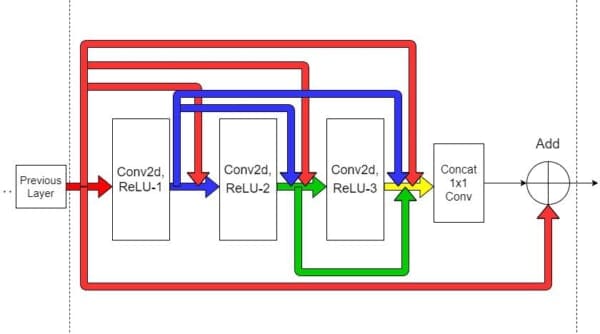
This way, the feedforward nature of the network is also preserved. Notice another important thing; the output from the previous layers has a direct link to all local connections within the present RDB. The simplest implication of this is that the information from a previous layer will always be available along with the present states, which enables our model to choose and prioritize from a variety of features adaptively. Thus, every bit of information is saved!

If you have heard about ResNets and Dense Blocks, Figure 2 might seem familiar as an RDB utilizes both concepts.

Let’s take a look at the code for the Residual Dense Block in subpixel_net.py.

# import the necessary packages
from . import config
from tensorflow.keras.layers import Add
from tensorflow.keras.layers import Conv2D
from tensorflow.keras.layers import Input
from tensorflow.keras.models import Model
import tensorflow as tf

def rdb_block(inputs, numLayers):
	# determine the number of channels present in the current input
	# and initialize a list with the current inputs for concatenation
	channels = inputs.get_shape()[-1]
	storedOutputs = [inputs]

We start with the rdb_block function (Line 9), which takes a layer input and the number of blocks as parameters. On Lines 12 and 13, we store the number of channels in a variable for later use, as well as create a list storedOutputs which will concatenate outputs as it encounters them.

	# iterate through the number of residual dense layers
	for _ in range(numLayers):
		# concatenate the previous outputs and pass it through a
		# CONV layer, and append the output to the ongoing concatenation
		localConcat = tf.concat(storedOutputs, axis=-1)
		out = Conv2D(filters=channels, kernel_size=3, padding="same",
			activation="relu",
			kernel_initializer="Orthogonal")(localConcat)
		storedOutputs.append(out)

Here, we have implemented the internal structure of an RDB. We are directly iterating through each of the layers present inside an RDB and storing each of the outputs. On Line 19, localConcat is acting as the link to each of the previous layers, as explained earlier. As we iterate through our given number of layers, localConcat encounters each of the previous outputs which were appended to the storedOutputs list at the end of each iteration (echoing a Dense block). On Lines 20-22, localConcat is then fed to the Conv2D layer.

	# concatenate all the outputs, pass it through a pointwise
	# convolutional layer, and add the outputs to initial inputs
	finalConcat = tf.concat(storedOutputs, axis=-1)
	finalOut = Conv2D(filters=inputs.get_shape()[-1], kernel_size=1,
		padding="same", activation="relu",
		kernel_initializer="Orthogonal")(finalConcat)
	finalOut = Add()([finalOut, inputs])

	# return the final output
	return finalOut

On Line 27, we concat all the previously stored outputs in storedOutputs and assign a new variable finalConcat to it. finalConcat is then fed to a Conv2D layer, thus completing the internal structure of an RDB. The final step on Line 31 is to add our initial input with our final concatenated output (echoing a Residual block). With that, we finish coding our Residual Dense Block. The number of layers within an RDB can be experimented with to see how the result is affected.

Next is our overall model architecture, where we will implement the Pixel Shuffle.

def get_subpixel_net(downsampleFactor=config.DOWN_FACTOR, channels=1,
	rdbLayers=config.RDB_LAYERS):
	# initialize an input layer
	inputs = Input((None, None, 1))

	# pass the inputs through a CONV => CONV block
	x = Conv2D(64, 5, padding="same", activation="relu",
		kernel_initializer="Orthogonal")(inputs)
	x = Conv2D(64, 3, padding="same", activation="relu",
		kernel_initializer="Orthogonal")(x)

	# pass the outputs through an RDB => CONV => RDB block
	x = rdb_block(x, numLayers=rdbLayers)
	x = Conv2D(32, 3, padding="same", activation="relu",
		kernel_initializer="Orthogonal")(x)
	x = rdb_block(x, numLayers=rdbLayers)

We start on Lines 37 and 38 by defining the arguments for get_subpixel_net, which is also our model function. The downsampling factor defined in config.py is necessary for us to know by what factor we need to upscale the image while the rdbBlocks argument uses the number of layers in a single block as set in config.py. We also have the argument channels, which is set as 1 by default since we had preprocessed the image to YUV format and isolated the Y channel.

The model architecture consists of adding two Conv2D layers (Lines 43-46) after which we invoke the rdb_block function as defined earlier (Line 49). This is followed by another Conv2D layer and an RDB block (Lines 50-52).

The next part of our code is where the magic happens. Before getting into it, let’s appreciate the folks at TensorFlow for giving us such a beautiful utility function called tf.nn.depth_to_space.

By its formal definition, it is a function that rearranges data from depth into blocks of spatial data. Understanding this is our key to debunking the mystery of Pixel Shuffle.

When we are talking about depth, we are referring to the number of channels in our tensor (speaking in image terms). So, if we have a tensor of shape 2, 2, 12 and we want to apply depth_to_space on it with a factor (also known as block_size) of 2, we have to see how the channel size is getting divided by block_size × block_size. So for channel size 12, we see that 12/(2×2) gives us the new channel size 3.

But since our channel size is reduced to 3, we obviously have to increase our height and width to maintain the overall size of the tensor as we are not losing data, just rearranging it. This gives us the final tensor shape of 4, 4, 3.

This phenomenon is what we term as pixel shuffle, where we are rearranging the elements of to .

	# pass the inputs through a final CONV layer such that the
	# channels of the outputs can be spatially organized into
	# the output resolution
	x = Conv2D(channels * (downsampleFactor ** 2), 3, padding="same",
		activation="relu", kernel_initializer="Orthogonal")(x)
	outputs = tf.nn.depth_to_space(x, downsampleFactor)

	# construct the final model and return it
	model = Model(inputs, outputs)
	return model

Notice how on Line 57, the Conv2D layer has its number of filters set as channels × downsampleFactor squared. We are essentially implementing the step before proceeding to use the tf.nn.depth_to_space (Line 59) function, where the tensor will be rearranged.

Note, even if this is our final output, tf.nn.depth_to_space is NOT a learnable parameter of the model. This means that the Conv2D layer right before it has to learn its upscaling filters properly so that the final output produces minimal loss during backpropagation.

Training the Pixel Shuffle Super-Resolution Model

With all the heavy lifting out of the way, all that is left for us is to train our model and test it on different images. For that, let’s move into the train.py module.

After importing the necessary package, we define a function called psnr, which takes an original image and a predicted image as its arguments. Our main intention is to calculate the Peak Signal to Noise Ratio (PSNR) by comparing the original and predicted images.

# USAGE
# python train.py

# import the necessary packages
from pyimagesearch.data_utils import process_input
from pyimagesearch import config
from pyimagesearch import subpixel_net
from imutils import paths
import matplotlib.pyplot as plt
import tensorflow as tf

def psnr(orig, pred):
	# cast the target images to integer
	orig = orig * 255.0
	orig = tf.cast(orig, tf.uint8)
	orig = tf.clip_by_value(orig, 0, 255)

	# cast the predicted images to integer
	pred = pred * 255.0
	pred = tf.cast(pred, tf.uint8)
	pred = tf.clip_by_value(pred, 0, 255)

	# return the psnr
	return tf.image.psnr(orig, pred, max_val=255)

Notice how on Lines 14-16 and Lines 19-21, we are upscaling the pixel values from the range [0.0, 1.0] to [0, 255]. The tensors are also getting cast into integers for easier calculations. For the PSNR calculations, we use the tf.image.psnr function (Line 24). As the name suggests, the higher the value of the ratio, the lower the value of the noise. The psnr function will also act as our model metric.

Our next task is to assign variables to the train and validation paths and create our train and validation datasets accordingly.

# define autotune flag for performance optimization
AUTO = tf.data.AUTOTUNE

# load the image paths from disk and initialize TensorFlow Dataset
# objects
print("[INFO] loading images from disk...")
trainPaths = list(paths.list_images(config.TRAIN_SET))
valPaths = list(paths.list_images(config.VAL_SET))
trainDS = tf.data.Dataset.from_tensor_slices(trainPaths)
valDS = tf.data.Dataset.from_tensor_slices(valPaths)

The paths.list_images function on Lines 32 and 33 gives us all the available images in a desired directory, which we are then passing on as a list to the tf.data.Dataset.from_tensor_slices function to initialize a TensorFlow Dataset Object (Lines 34 and 35).

Next, we create the train and validation data loaders and compile our model.

# prepare data loaders
print("[INFO] preparing data loaders...")
trainDS = trainDS.map(process_input,
					  num_parallel_calls=AUTO).batch(
	config.BATCH_SIZE).prefetch(AUTO)
valDS = valDS.map(process_input,
				  num_parallel_calls=AUTO).batch(
	config.BATCH_SIZE).prefetch(AUTO)

# initialize, compile, and train the model
print("[INFO] initializing and training model...")
model = subpixel_net.get_subpixel_net()
model.compile(optimizer="adam", loss="mse", metrics=psnr)
H = model.fit(trainDS, validation_data=valDS, epochs=config.EPOCHS)

On Lines 39-44, we are using the tf.data.Dataset.map function to map our dataset elements to a function and return a new dataset. The function we are using is process_input, which we had defined in the data_utils module. Thus, our train and validation data loaders are ready.

As you can see on Line 49, we are using psnr as our model metric, which means the goal of our model will be to maximize the Peak Signal to Noise Ratio. We use the adam optimizer and choose mse (mean squared error) as our loss function. On Line 50, we proceed to fit our model with the data loaders.

# prepare training plot of the model and serialize it
plt.style.use("ggplot")
plt.figure()
plt.plot(H.history["loss"], label="train_loss")
plt.plot(H.history["val_loss"], label="val_loss")
plt.plot(H.history["psnr"], label="train_psnr")
plt.plot(H.history["val_psnr"], label="val_psnr")
plt.title("Training Loss and PSNR")
plt.xlabel("Epoch #")
plt.ylabel("Loss/PSNR")
plt.legend(loc="lower left")
plt.savefig(config.TRAINING_PLOT)

# serialize the trained model
print("[INFO] serializing model...")
model.save(config.SUPER_RES_MODEL)

On Lines 53-63, we plot a few graphs to assess how well our model fared. Our model is now ready, and we will use it on some test images to see what the results are. So, don’t forget to save your model (Line 67)!

Training Results and Loss Visualization

Upon execution of the file train.py, our model gets trained. Below is the epoch-wise training history of the model which will be fully available to you once you run the module.

$ python train.py
[INFO] loading images from disk...
[INFO] preparing data loaders...
[INFO] initializing and training model...
Epoch 1/100
25/25 [==============================] - 4s 65ms/step - loss: 0.0859 - psnr: 11.9725 - val_loss: 0.0105 - val_psnr: 18.9549
Epoch 2/100
25/25 [==============================] - 1s 42ms/step - loss: 0.0084 - psnr: 20.2418 - val_loss: 0.0064 - val_psnr: 20.6150
Epoch 3/100
25/25 [==============================] - 1s 42ms/step - loss: 0.0055 - psnr: 22.3704 - val_loss: 0.0043 - val_psnr: 22.2737
...
Epoch 98/100
25/25 [==============================] - 1s 42ms/step - loss: 0.0019 - psnr: 27.2354 - val_loss: 0.0021 - val_psnr: 26.2384
Epoch 99/100
25/25 [==============================] - 1s 42ms/step - loss: 0.0019 - psnr: 27.2533 - val_loss: 0.0021 - val_psnr: 25.9284
Epoch 100/100
25/25 [==============================] - 1s 42ms/step - loss: 0.0019 - psnr: 27.2359 - val_loss: 0.0021 - val_psnr: 25.9741
[INFO] serializing model...

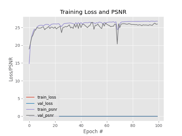
So, we reach a final validation loss of 0.0021 and a validation PSNR score of 25.9741.

Figure 3 displays the Training History Curve showing the Training Loss and PSNR Score at different epochs.

Generating Super-Resolution Images with Pixel Shuffle

Since our model training is over, let’s discuss a few things. The graphs and scores of our model suggest that the use of RDBs does not significantly boost PSNR stats. So, where does our model excel? Let’s test it out and see for ourselves.

To finally generate the images by applying super resolution using the trained Sub-pixel CNN with RDB, let’s open the generate_super_res.py and start coding.

# USAGE
# python generate_super_res.py

# import the necessary packages
from pyimagesearch import config
from PIL import Image
from tensorflow.keras.preprocessing.image import load_img
from tensorflow.keras.models import load_model
from imutils import paths
import matplotlib.pyplot as plt
import tensorflow as tf
import numpy as np
 

def psnr(orig, pred):
	# cast the target images to integer
	orig = orig * 255.0
	orig = tf.cast(orig, tf.uint8)
	orig = tf.clip_by_value(orig, 0, 255)

	# cast the predicted images to integer
	pred = pred * 255.0
	pred = tf.cast(pred, tf.uint8)
	pred = tf.clip_by_value(pred, 0, 255)

	# return the psnr
	return tf.image.psnr(orig, pred, max_val=255)

We start on Line 15 by defining another function psnr, which calculates the PSNR of the predicted output and original image. As mentioned earlier, a higher PSNR indicates a better result.

def load_image(imagePath):
	# load image from disk and downsample it using the bicubic method
	orig = load_img(imagePath)
	downsampled = orig.resize((orig.size[0] // config.DOWN_FACTOR,
		orig.size[1] // config.DOWN_FACTOR), Image.BICUBIC)

	# return a tuple of the original and downsampled image
	return (orig, downsampled)

On Line 29, we write a helper function load_image, which takes the image path as its argument and returns the original and downsampled images. Notice that on Lines 32 and 33, we are downsampling the images according to our DOWN_FACTOR which was defined in the config.py module. This is a very important step, as our model’s output dimensions depend on this.

def get_y_channel(image):
	# convert the image to YCbCr colorspace and then split it to get the
	# individual channels
	ycbcr = image.convert("YCbCr")
	(y, cb, cr) = ycbcr.split()

	# convert the y-channel to a numpy array, cast it to float, and
	# scale its pixel range to [0, 1]
	y = np.array(y)
	y = y.astype("float32") / 255.0

	# return a tuple of the individual channels
	return (y, cb, cr)

Next, we define a function called get_y_channel, which converts the RGB image to its equivalent YCbCr form to isolate the Y channel. In accordance with something we have maintained throughout our blog, we scale the values of the pixels to the range of [0.0, 1.0] (Line 47), before passing it through our model.

def clip_numpy(image):
	# cast image to integer, clip its pixel range to [0, 255]
	image = tf.cast(image * 255.0, tf.uint8)
	image = tf.clip_by_value(image, 0, 255).numpy()

	# return the image
	return image

Lines 52-58 contain our final minor helper function clip_numpy, which clips the values of the image based on the given range. Since this function is a part of our post-processing step, we are going to upscale the range to [0, 255] again from [0.0, 1.0] (Line 54) and clip any values beyond the given boundaries (Line 55).

def postprocess_image(y, cb, cr):
	# do a bit of initial preprocessing, reshape it to match original
	# size, and then convert it to a PIL Image
	y = clip_numpy(y).squeeze()
	y = y.reshape(y.shape[0], y.shape[1])
	y = Image.fromarray(y, mode="L")

	# resize the other channels of the image to match the original
	# dimension
	outputCB= cb.resize(y.size, Image.BICUBIC)
	outputCR= cr.resize(y.size, Image.BICUBIC)

	# merge the resized channels altogether and return it as a numpy
	# array
	final = Image.merge("YCbCr", (y, outputCB, outputCR)).convert("RGB")
	return np.array(final)

Here, let me remind you that our model only works with the Y channel and hence will also output a Y channel. Lines 60-75 contain the postprocess_image which will convert our predicted result into an RGB image.

With all our utility functions done, we can finally move on to generating some super-resolution images. We create a variable called testPaths which will contain the paths of all the available test images. A second variable currentTestPaths will randomly choose 10 values between the available test paths every time it’s called. We also load our previously saved model.

# load the test image paths from disk and select ten paths randomly
print("[INFO] loading test images...")
testPaths = list(paths.list_images(config.TEST_SET))
currentTestPaths = np.random.choice(testPaths, 10)

# load our super-resolution model from disk
print("[INFO] loading model...")
superResModel = load_model(config.SUPER_RES_MODEL,
	custom_objects={"psnr" : psnr})

Iterating through the available test image paths in currentTestPaths (Line 80), we pass the image through our model and compare the prediction with an image resized using the Naive Bicubic method (one of the old techniques used for upscaling images).

# iterate through our test image paths
print("[INFO] performing predictions...")
for (i, path) in enumerate(currentTestPaths):
	# grab the original and the downsampled images from the
	# current path
	(orig, downsampled) = load_image(path)

	# retrieve the individual channels of the current image and perform
	# inference
	(y, cb, cr) = get_y_channel(downsampled)
	upscaledY = superResModel.predict(y[None, ...])[0]

	# postprocess the output and apply the naive bicubic resizing to
	# the downsampled image for comparison
	finalOutput = postprocess_image(upscaledY, cb, cr)
	naiveResizing = downsampled.resize(orig.size, Image.BICUBIC)

	# visualize the results and save them to disk
	path = os.path.join(config.VISUALIZATION_PATH, f"{i}_viz.png")
	(fig, (ax1, ax2)) = plt.subplots(ncols=2, figsize=(12, 12))
	ax1.imshow(naiveResizing)
	ax2.imshow(finalOutput.astype("int"))
	ax1.set_title("Naive Bicubic Resizing")
	ax2.set_title("Super-res Model")
	fig.savefig(path, dpi=300, bbox_inches="tight")

Once inside the loop, we start on Line 92 by passing the path in the current iteration to the load_image function, followed by the get_y_channel function to isolate the Y channel. On Line 97, we pass the isolated Y channel to our super-resolution model. Notice how the format is superResModel.predict(y)[0]. That is because we only need the value of the first element of the list that the model outputs. We pass the predicted output through the postprocess_image function.

We are done with the code for inference. On Line 105, we are referencing our directory which was created to save visualizations. Now it’s time to go through the plots generated by Lines 106-111.

Visualizing the Generated Super-Resolution Images

With all the coding out of the way, all we are left to do is run the python generate_super_res.py command in the shell script.

$ python generate_super_res.py
[INFO] loading test images...
[INFO] loading model...
[INFO] performing predictions...

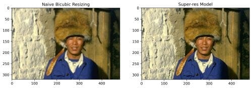
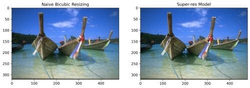
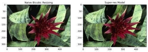
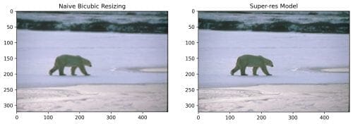
As mentioned before, using Residual Dense Blocks didn’t have any significant effect on the PSNR stats. However, upon visualization of the images (Figures 4-7), we see how superior they are in visual quality compared to the Naive Bicubic method. A subtle conclusion can be drawn from these visualizations; the RDNs learned hierarchical features well enough for the image to be upscaled with such a commendable visual quality.

Summary

In this tutorial, we learned a way to implement super resolution with the help of an Efficient Sub-pixel CNN fitted with Residual Dense Blocks. Along the way, we also encountered several beautiful concepts that are used in the implementation.

In the end, we observed that the sub-pixel CNN yielded almost the same quality images as that of the original. Readers are encouraged to tinker around with the parameters (e.g., the number of layers inside an RDB) to see how the results are affected. Do tag PyImageSearch (@PyImageSearch) when you share your results with the world!

Citation Information

Chakraborty, D. “Pixel shuffle super resolution with TensorFlow, Keras, and deep learning,” PyImageSearch, 2021, https://pyimagesearch.com/2021/09/27/pixel-shuffle-super-resolution-with-tensorflow-keras-and-deep-learning/

@article{dev2021, author = {Devjyoti Chakraborty}, title = {Pixel Shuffle Super Resolution with {TensorFlow}, {K}eras, and Deep Learning}, journal = {PyImageSearch}, year = {2021}, note = {https://pyimagesearch.com/2021/09/27/pixel-shuffle-super-resolution-with-tensorflow-keras-and-deep-learning/}, }

To download the source code to this post (and be notified when future tutorials are published here on PyImageSearch), simply enter your email address in the form below!