Fine-tuning ResNet with Keras, TensorFlow, and Deep Learning

In this tutorial, you will learn how to fine-tune ResNet using Keras, TensorFlow, and Deep Learning.

A couple of months ago, I posted on Twitter asking my followers for help creating a dataset of camouflage vs. noncamouflage clothes:

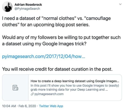
This dataset was to be used on a special project that Victor Gevers, an esteemed ethical hacker from the GDI.Foundation, and I were working on (more on that in two weeks, when I’ll reveal the details on what we’ve built).

Two PyImageSearch readers, Julia Riede and Nitin Rai, not only stepped up to the plate to help out but hit a home run!

Both of them spent a couple of days downloading images for each class, organizing the files, and then uploading them so Victor and I could train a model on them — thank you so much, Julia and Nitin; we couldn’t have done it without you!

A few days after I started working with the camouflage vs. noncamouflage dataset, I received an email from PyImageSearch reader Lucas:

Hi Adrian, I’m big fan of the PyImageSearch blog. It’s helped me tremendously with my undergrad project.

I have a question for you:

Do you have any tutorials on how to fine-tune ResNet?

I’ve been going through your archives and it seems like you’ve covered fine-tuning other architectures (ex. VGGNet) but I couldn’t find anything on ResNet. I’ve been trying to fine-tune ResNet with Keras/TensorFlow for the past few days and I just keep running into errors.

If you can help me out I would appreciate it.

I was already planning on fine-tuning a model on top of the camouflage vs. noncamouflage clothes dataset, so helping Lucas seemed like a natural fit.

Inside the remainder of this this tutorial you will:

1. Discover the seminal ResNet architecture
2. Learn how to fine-tune it using Keras and TensorFlow
3. Fine-tune ResNet for camouflage vs. noncamouflage clothes detection

And in two weeks, I’ll show you the practical, real-world use case that Victor and I applied camouflage detection to — it’s a great story, and you won’t want to miss it!

To learn how to fine-tune ResNet with Keras and TensorFlow, just keep reading!

Fine-tuning ResNet with Keras, TensorFlow, and Deep Learning

In the first part of this tutorial, you will learn about the ResNet architecture, including how we can fine-tune ResNet using Keras and TensorFlow.

From there, we’ll discuss our camouflage clothing vs. normal clothing image dataset in detail.

We’ll then review our project directory structure and proceed to:

1. Implement our configuration file
2. Create a Python script to build/organize our image dataset
3. Implement a second Python script used to fine-tune ResNet with Keras and TensorFlow
4. Execute the training script and fine-tune ResNet on our dataset

Let’s get started!

What is ResNet?

ResNet was first introduced by He et al. in their seminal 2015 paper, Deep Residual Learning for Image Recognition — that paper has been cited an astonishing 43,064 times!

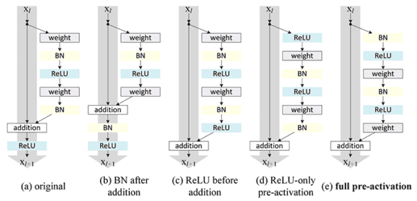
A follow-up paper in 2016, Identity Mappings in Deep Residual Networks, performed a series of ablation experiments, playing with the inclusion, removal, and ordering of various components in the residual module, ultimately resulting in a variation of ResNet that:

1. Is easier to train
2. Is more tolerant of hyperparameters, including regularization and initial learning rate
3. Generalizes better

ResNet is arguably the most important network architecture since:

• AlexNet — which reignited researcher interest in deep neural networks back in 2012
• VGGNet — which demonstrated how deeper neural networks could be trained successfully using only 3×3 convolutions (2014)
• GoogLeNet — which introduced the inception module/micro-architecture (2014)

In fact, the techniques that ResNet employs have been successfully applied to noncomputer vision tasks, including audio classification and Natural Language Processing (NLP)!

How does ResNet work?

Note: The following section was adapted from Chapter 12 of my book, Deep Learning for Computer Vision with Python (Practitioner Bundle).

The original residual module introduced by He et al. relies on the concept of identify mappings, the process of taking the original input to the module and adding it to the output of a series of operations:

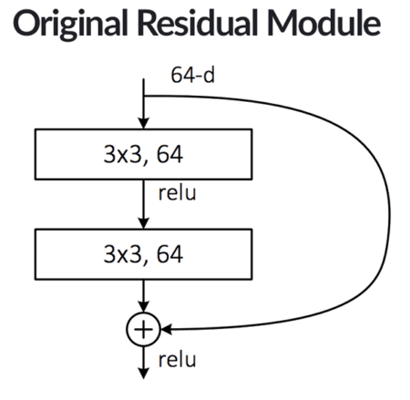
At the top of the module, we accept an input to the module (i.e., the previous layer in the network). The right branch is a “linear shortcut” — it connects the input to an addition operation at the bottom of the model. Then, on the left branch of the residual module, we apply a series of convolutions (both of which are 3×3), activations, and batch normalizations. This is a standard pattern to follow when constructing Convolutional Neural Networks.

But what makes ResNet interesting is that He et al. suggested adding the original input to the output of the CONV, RELU, and BN layers.

We call this addition an identity mapping since the input (the identity) is added to the output of a series of operations.

It’s also way the term residual is used — the “residual” input is added to the output of a series of layer operations. The connection between the input and addition node is called the shortcut.

While traditional neural networks can be seen as learning a function y = f(x), a residual layer attempts to approximate y via f(x) + id(x) = f(x) + x where id(x) is the identity function.

These residual layers start at the identity function and evolve to become more complex as the network learns. This type of residual learning framework allows us to train networks that are substantially deeper than previously proposed architectures.

Furthermore, since the input is included in every residual module, it turns out the network can learn faster and with larger learning rates.

In the original 2015 paper, He et al. also included an extension to the original residual module called bottlenecks:

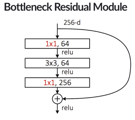
Here we can see that the same identity mapping is taking place, only now the CONV layers in the left branch of the residual module have been updated:

1. We are utilizing three CONV layers rather than just two
2. The first and last CONV layers are 1×1 convolutions
3. The number of filters learned in the first two CONV layers are 1/4 the number of filters learned in the final CONV

This variation of the residual module serves as a form of dimensionality reduction, thereby reducing the total number of parameters in the network (and doing so without sacrificing accuracy). This form of dimensionality reduction is called the bottleneck.

He et al.’s 2016 publication on Identity Mappings in Deep Residual Networks performed a series of ablation studies, playing with the inclusion, removal, and ordering of various components in the residual module, ultimately resulting in the concept of pre-activation:

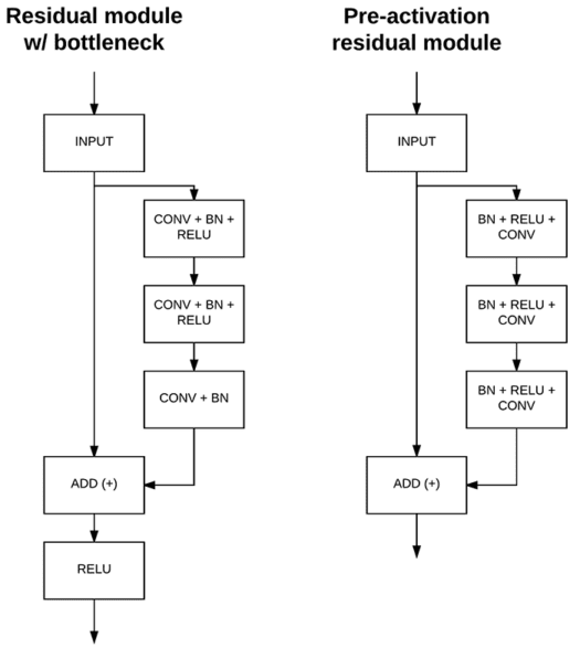
Without going into too much detail, the pre-activation residual module rearranges the order in which convolution, batch normalization, and activation are performed.

The original residual module (with bottleneck) accepts an input (i.e., a RELU activation map) and then applies a series of (CONV => BN => RELU) * 2 => CONV => BN before adding this output to the original input and applying a final RELU activation.

Their 2016 study demonstrated that instead, applying a series of (BN => RELU => CONV) * 3 led to higher accuracy models that were easier to train.

We call this method of layer ordering pre-activation as our RELUs and batch normalizations are placed before the convolutions, which is in contrast to the typical approach of applying RELUs and batch normalizations after the convolutions.

For a more complete review of ResNet, including how to implement it from scratch using Keras/TensorFlow, be sure to refer to my book, Deep Learning for Computer Vision with Python.

How can we fine-tune it with Keras and TensorFlow?

In order to fine-tune ResNet with Keras and TensorFlow, we need to load ResNet from disk using the pre-trained ImageNet weights but leaving off the fully-connected layer head.

We can do so using the following code:

>>> baseModel = ResNet50(weights="imagenet", include_top=False,
	input_tensor=Input(shape=(224, 224, 3)))

Inspecting the baseModel.summary(), you’ll see the following:

...
conv5_block3_3_conv (Conv2D)    (None, 7, 7, 2048)   1050624     conv5_block3_2_relu[0][0]        
__________________________________________________________________________________________________
conv5_block3_3_bn (BatchNormali (None, 7, 7, 2048)   8192        conv5_block3_3_conv[0][0]        
__________________________________________________________________________________________________
conv5_block3_add (Add)          (None, 7, 7, 2048)   0           conv5_block2_out[0][0]           
                                                                 conv5_block3_3_bn[0][0]          
__________________________________________________________________________________________________
conv5_block3_out (Activation)   (None, 7, 7, 2048)   0           conv5_block3_add[0][0]           
==================================================================================================

Here, we can observe that the final layer in the ResNet architecture (again, without the fully-connected layer head) is an Activation layer that is 7 x 7 x 2048.

We can construct a new, freshly initialized layer head by accepting the baseModel.output and then applying a 7×7 average pooling, followed by our fully-connected layers:

headModel = baseModel.output
headModel = AveragePooling2D(pool_size=(7, 7))(headModel)
headModel = Flatten(name="flatten")(headModel)
headModel = Dense(256, activation="relu")(headModel)
headModel = Dropout(0.5)(headModel)
headModel = Dense(len(config.CLASSES), activation="softmax")(headModel)

With the headModel constructed, we simply need to append it to the body of the ResNet model:

model = Model(inputs=baseModel.input, outputs=headModel)

Now, if we take a look at the model.summary(), we can conclude that we have successfully added a new fully-connected layer head to ResNet, making the architecture suitable for fine-tuning:

conv5_block3_3_conv (Conv2D)    (None, 7, 7, 2048)   1050624     conv5_block3_2_relu[0][0]        
__________________________________________________________________________________________________
conv5_block3_3_bn (BatchNormali (None, 7, 7, 2048)   8192        conv5_block3_3_conv[0][0]        
__________________________________________________________________________________________________
conv5_block3_add (Add)          (None, 7, 7, 2048)   0           conv5_block2_out[0][0]           
                                                                 conv5_block3_3_bn[0][0]          
__________________________________________________________________________________________________
conv5_block3_out (Activation)   (None, 7, 7, 2048)   0           conv5_block3_add[0][0]           
__________________________________________________________________________________________________
average_pooling2d (AveragePooli (None, 1, 1, 2048)   0           conv5_block3_out[0][0]           
__________________________________________________________________________________________________
flatten (Flatten)               (None, 2048)         0           average_pooling2d[0][0]          
__________________________________________________________________________________________________
dense (Dense)                   (None, 256)          524544      flatten[0][0]                    
__________________________________________________________________________________________________
dropout (Dropout)               (None, 256)          0           dense[0][0]                      
__________________________________________________________________________________________________
dense_1 (Dense)                 (None, 2)            514         dropout[0][0]                    
==================================================================================================

In the remainder of this tutorial, I will provide you with a fully working example of fine-tuning ResNet using Keras and TensorFlow.

Our camouflage vs. normal clothing dataset

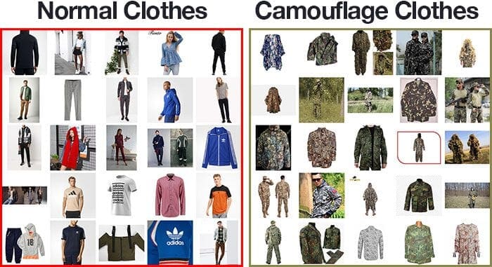
In this tutorial, we will be training a camouflage clothes vs. normal clothes detector.

I’ll be discussing exactly why we’re building a camouflage clothes detector in two weeks, but for the time being, let this serve as a standalone example of how to fine-tune ResNet with Keras and TensorFlow.

The dataset we’re using here was curated by PyImageSearch readers, Julia Riede and Nitin Rai.

The dataset consists of two classes, each with an equal number of images:

• camouflage_clothes: 7,949 images
• normal_clothes: 7,949 images

A sample of the images for each class can be seen in Figure 6.

In the remainder of this tutorial, you’ll learn how to fine-tune ResNet to predict both of these classes — the knowledge that you gain will enable you to fine-tune ResNet on your own datasets as well.

Downloading our camouflage vs. normal clothing dataset

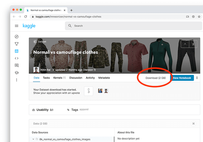
The camouflage clothes vs. normal clothes dataset can be downloaded directly from Kaggle:

https://www.kaggle.com/imneonizer/normal-vs-camouflage-clothes

Simply click the “Download” button (Figure 7) to download a .zip archive of the dataset.

Project structure

Be sure to grab and unzip the code from the “Downloads” section of this blog post. Let’s take a moment to inspect the organizational structure of our project:

$ tree --dirsfirst --filelimit 10
.
├── 8k_normal_vs_camouflage_clothes_images
│   ├── camouflage_clothes [7949 entries]
│   └── normal_clothes [7949 entries]
├── pyimagesearch
│   ├── __init__.py
│   └── config.py
├── build_dataset.py
├── camo_detector.model
├── normal-vs-camouflage-clothes.zip
├── plot.png
└── train_camo_detector.py

4 directories, 7 files

As you can see, I’ve placed the dataset (normal-vs-camouflage-clothes.zip) in the root directory of our project and extracted the files. The images therein now reside in the 8k_normal_vs_camouflage_clothes_images directory.

Today’s pyimagesearch module comes with a single Python configuration file (config.py) that houses our important paths and variables. We’ll review this file in the next section.

Our Python driver scripts consist of:

• build_dataset.py: Splits our data into training, testing, and validation subdirectories
• train_camo_detector.py: Trains a camouflage classifier with Python, TensorFlow/Keras, and fine-tuning

Our configuration file

Before we can (1) build our camouflage vs. noncamouflage image dataset and (2) fine-tune ResNet on our image dataset, let’s first create a simple configuration file to store all our important image paths and variables.

Open up the config.py file in your project, and insert the following code:

# import the necessary packages
import os

# initialize the path to the *original* input directory of images
ORIG_INPUT_DATASET = "8k_normal_vs_camouflage_clothes_images"

# initialize the base path to the *new* directory that will contain
# our images after computing the training and testing split
BASE_PATH = "camo_not_camo"

# derive the training, validation, and testing directories
TRAIN_PATH = os.path.sep.join([BASE_PATH, "training"])
VAL_PATH = os.path.sep.join([BASE_PATH, "validation"])
TEST_PATH = os.path.sep.join([BASE_PATH, "testing"])

The os module import allows us to build dynamic paths directly in our configuration file.

Our existing input dataset path should be placed on Line 5 (the Kaggle dataset you should have downloaded by this point).

The path to our new dataset directory that will contain our training, testing, and validation splits is shown on Line 9. This path will be created by the build_dataset.py script.

Three subdirectories per class (we have two classes) will also be created (Lines 12-14) — the paths to our training, validation, and testing dataset splits. Each will be populated with a subset of the images from our dataset.

Next, we’ll define our split percentages and classes:

# define the amount of data that will be used training
TRAIN_SPLIT = 0.75

# the amount of validation data will be a percentage of the
# *training* data
VAL_SPLIT = 0.1

# define the names of the classes
CLASSES = ["camouflage_clothes", "normal_clothes"]

Training data will be represented by 75% of all the data available (Line 17), 10% of which will be marked for validation (Line 21).

Our camouflage and normal clothes classes are defined on Line 24.

We’ll wrap up with a few hyperparameters and our output model path:

# initialize the initial learning rate, batch size, and number of
# epochs to train for
INIT_LR = 1e-4
BS = 32
NUM_EPOCHS = 20

# define the path to the serialized output model after training
MODEL_PATH = "camo_detector.model"

The initial learning rate, batch size, and number of epochs to train for are set on Lines 28-30.

The path to the output serialized ResNet-based camouflage classification model after fine-tuning will be stored at the path defined on Line 33.

Implementing our camouflage dataset builder script

With our configuration file implemented, let’s move on to creating our dataset builder, which will:

1. Split our dataset into training, validation, and testing sets, respectively
2. Organize our images on disk so we can use Keras’ ImageDataGenerator class and associated flow_from_directory function to easily fine-tune ResNet

Open up build_dataset.py, and let’s get started:

# import the necessary packages
from pyimagesearch import config
from imutils import paths
import random
import shutil
import os

We begin by importing our config from the previous section along with the paths module, which will help us to find the image files on disk. Three modules built into Python will be used for shuffling paths and creating directories/subdirectories.

Let’s go ahead and grab the paths to all original images in our dataset:

# grab the paths to all input images in the original input directory
# and shuffle them
imagePaths = list(paths.list_images(config.ORIG_INPUT_DATASET))
random.seed(42)
random.shuffle(imagePaths)

# compute the training and testing split
i = int(len(imagePaths) * config.TRAIN_SPLIT)
trainPaths = imagePaths[:i]
testPaths = imagePaths[i:]

# we'll be using part of the training data for validation
i = int(len(trainPaths) * config.VAL_SPLIT)
valPaths = trainPaths[:i]
trainPaths = trainPaths[i:]

# define the datasets that we'll be building
datasets = [
	("training", trainPaths, config.TRAIN_PATH),
	("validation", valPaths, config.VAL_PATH),
	("testing", testPaths, config.TEST_PATH)
]

Lines 25-29 define the dataset splits we’ll be building in the remainder of this script. Let’s proceed:

# loop over the datasets
for (dType, imagePaths, baseOutput) in datasets:
	# show which data split we are creating
	print("[INFO] building '{}' split".format(dType))

	# if the output base output directory does not exist, create it
	if not os.path.exists(baseOutput):
		print("[INFO] 'creating {}' directory".format(baseOutput))
		os.makedirs(baseOutput)

	# loop over the input image paths
	for inputPath in imagePaths:
		# extract the filename of the input image along with its
		# corresponding class label
		filename = inputPath.split(os.path.sep)[-1]
		label = inputPath.split(os.path.sep)[-2]

		# build the path to the label directory
		labelPath = os.path.sep.join([baseOutput, label])

		# if the label output directory does not exist, create it
		if not os.path.exists(labelPath):
			print("[INFO] 'creating {}' directory".format(labelPath))
			os.makedirs(labelPath)

		# construct the path to the destination image and then copy
		# the image itself
		p = os.path.sep.join([labelPath, filename])
		shutil.copy2(inputPath, p)

This last block of code handles copying images from their original location into their destination path; directories and subdirectories are created in the process. Let’s review in more detail:

• We loop over each of the datasets, creating the directory if it doesn’t exist (Lines 32-39)
• For each of our imagePaths, we proceed to:
  • Extract the filename and class label (Lines 45 and 46)
  • Build the path to the label directory (Line 49) and create the subdirectory, if required (Lines 52-54)
  • Copy the image from the source directory into its destination (Lines 58 and 59)

In the next section, we’ll build our dataset accordingly.

Building the camouflage image dataset

Let’s now build and organize our image camouflage dataset.

Make sure you have:

1. Used the “Downloads” section of this tutorial to download the source code
2. Followed the “Downloading our camouflage vs. normal clothing dataset” section above to download the dataset

From there, open a terminal, and execute the following command:

$ python build_dataset.py
[INFO] building 'training' split
[INFO] 'creating camo_not_camo/training' directory
[INFO] 'creating camo_not_camo/training/normal_clothes' directory
[INFO] 'creating camo_not_camo/training/camouflage_clothes' directory
[INFO] building 'validation' split
[INFO] 'creating camo_not_camo/validation' directory
[INFO] 'creating camo_not_camo/validation/camouflage_clothes' directory
[INFO] 'creating camo_not_camo/validation/normal_clothes' directory
[INFO] building 'testing' split
[INFO] 'creating camo_not_camo/testing' directory
[INFO] 'creating camo_not_camo/testing/normal_clothes' directory
[INFO] 'creating camo_not_camo/testing/camouflage_clothes' directory

You can then use the tree command to inspect camo_not_camo directory to validate that each of the training, testing, and validation splits was created:

$ tree camo_not_camo --filelimit 20
camo_not_camo
├── testing
│   ├── camouflage_clothes [2007 entries]
│   └── normal_clothes [1968 entries]
├── training
│   ├── camouflage_clothes [5339 entries]
│   └── normal_clothes [5392 entries]
└── validation
    ├── camouflage_clothes [603 entries]
    └── normal_clothes [589 entries]

9 directories, 0 files

Implementing our ResNet fine-tuning script with Keras and TensorFlow

With our dataset created and properly organized on disk, let’s learn how we can fine-tune ResNet using Keras and TensorFlow.

Open the train_camo_detector.py file, and insert the following code:

# set the matplotlib backend so figures can be saved in the background
import matplotlib
matplotlib.use("Agg")

# import the necessary packages
from pyimagesearch import config
from tensorflow.keras.preprocessing.image import ImageDataGenerator
from tensorflow.keras.layers import AveragePooling2D
from tensorflow.keras.layers import Dropout
from tensorflow.keras.layers import Flatten
from tensorflow.keras.layers import Dense
from tensorflow.keras.layers import Input
from tensorflow.keras.models import Model
from tensorflow.keras.optimizers import Adam
from tensorflow.keras.applications import ResNet50
from sklearn.metrics import classification_report
from imutils import paths
import matplotlib.pyplot as plt
import numpy as np
import argparse

# construct the argument parser and parse the arguments
ap = argparse.ArgumentParser()
ap.add_argument("-p", "--plot", type=str, default="plot.png",
	help="path to output loss/accuracy plot")
args = vars(ap.parse_args())

# determine the total number of image paths in training, validation,
# and testing directories
totalTrain = len(list(paths.list_images(config.TRAIN_PATH)))
totalVal = len(list(paths.list_images(config.VAL_PATH)))
totalTest = len(list(paths.list_images(config.TEST_PATH)))

We have a single command line argument --plot, the path to an image file that will have our accuracy/loss training curves. Our other configurations are in the Python configuration file we reviewed previously.

Lines 30-32 determine the total number of training, validation, and testing images, respectively.

Next, we’ll prepare for data augmentation:

# initialize the training training data augmentation object
trainAug = ImageDataGenerator(
	rotation_range=25,
	zoom_range=0.1,
	width_shift_range=0.1,
	height_shift_range=0.1,
	shear_range=0.2,
	horizontal_flip=True,
	fill_mode="nearest")

# initialize the validation/testing data augmentation object (which
# we'll be adding mean subtraction to)
valAug = ImageDataGenerator()

# define the ImageNet mean subtraction (in RGB order) and set the
# the mean subtraction value for each of the data augmentation
# objects
mean = np.array([123.68, 116.779, 103.939], dtype="float32")
trainAug.mean = mean
valAug.mean = mean

Data augmentation allows for training time mutations of our images including random rotations, zooms, shifts, shears, flips, and mean subtraction. Lines 35-42 initialize our training data augmentation object with a selection of these parameters. Similarly, Line 46 initializes the validation/testing data augmentation object (it will only be used for mean subtraction).

Both of our data augmentation objects are set up to perform mean subtraction on-the-fly (Lines 51-53).

We’ll now instantiate three Python generators from our data augmentation objects:

# initialize the training generator
trainGen = trainAug.flow_from_directory(
	config.TRAIN_PATH,
	class_mode="categorical",
	target_size=(224, 224),
	color_mode="rgb",
	shuffle=True,
	batch_size=config.BS)

# initialize the validation generator
valGen = valAug.flow_from_directory(
	config.VAL_PATH,
	class_mode="categorical",
	target_size=(224, 224),
	color_mode="rgb",
	shuffle=False,
	batch_size=config.BS)

# initialize the testing generator
testGen = valAug.flow_from_directory(
	config.TEST_PATH,
	class_mode="categorical",
	target_size=(224, 224),
	color_mode="rgb",
	shuffle=False,
	batch_size=config.BS)

Let’s load our ResNet50 classification model and prepare it for fine-tuning:

# load the ResNet-50 network, ensuring the head FC layer sets are left
# off
print("[INFO] preparing model...")
baseModel = ResNet50(weights="imagenet", include_top=False,
	input_tensor=Input(shape=(224, 224, 3)))

# construct the head of the model that will be placed on top of the
# the base model
headModel = baseModel.output
headModel = AveragePooling2D(pool_size=(7, 7))(headModel)
headModel = Flatten(name="flatten")(headModel)
headModel = Dense(256, activation="relu")(headModel)
headModel = Dropout(0.5)(headModel)
headModel = Dense(len(config.CLASSES), activation="softmax")(headModel)

# place the head FC model on top of the base model (this will become
# the actual model we will train)
model = Model(inputs=baseModel.input, outputs=headModel)

# loop over all layers in the base model and freeze them so they will
# *not* be updated during the training process
for layer in baseModel.layers:
	layer.trainable = False

The final step for fine-tuning is to ensure that the weights of the base of our CNN are frozen (Lines 103 and 104) — we only want to train (i.e., fine-tune) the head of the network.

If you need to brush up on the concept of fine-tuning, please refer to my fine-tuning articles, in particular Fine-tuning with Keras and Deep Learning.

We’re now ready to fine-tune our ResNet-based camouflage detector with TensorFlow, Keras, and deep learning:

# compile the model
opt = Adam(lr=config.INIT_LR, decay=config.INIT_LR / config.NUM_EPOCHS)
model.compile(loss="binary_crossentropy", optimizer=opt,
	metrics=["accuracy"])

# train the model
print("[INFO] training model...")
H = model.fit_generator(
	trainGen,
	steps_per_epoch=totalTrain // config.BS,
	validation_data=valGen,
	validation_steps=totalVal // config.BS,
	epochs=config.NUM_EPOCHS)

First, we compile our model with learning rate decay and the Adam optimizer using "binary_crossentropy" loss, since this is a two-class problem (Lines 107-109). If you are training with more than two classes of data, be sure to set your loss to "categorical_crossentropy".

Lines 113-118 then train our model using our training and validation data generators.

Upon the completion of training, we’ll evaluate our model on the testing set:

# reset the testing generator and then use our trained model to
# make predictions on the data
print("[INFO] evaluating network...")
testGen.reset()
predIdxs = model.predict_generator(testGen,
	steps=(totalTest // config.BS) + 1)

# for each image in the testing set we need to find the index of the
# label with corresponding largest predicted probability
predIdxs = np.argmax(predIdxs, axis=1)

# show a nicely formatted classification report
print(classification_report(testGen.classes, predIdxs,
	target_names=testGen.class_indices.keys()))

# serialize the model to disk
print("[INFO] saving model...")
model.save(config.MODEL_PATH, save_format="h5")

# plot the training loss and accuracy
N = config.NUM_EPOCHS
plt.style.use("ggplot")
plt.figure()
plt.plot(np.arange(0, N), H.history["loss"], label="train_loss")
plt.plot(np.arange(0, N), H.history["val_loss"], label="val_loss")
plt.plot(np.arange(0, N), H.history["accuracy"], label="train_acc")
plt.plot(np.arange(0, N), H.history["val_accuracy"], label="val_acc")
plt.title("Training Loss and Accuracy on Dataset")
plt.xlabel("Epoch #")
plt.ylabel("Loss/Accuracy")
plt.legend(loc="lower left")
plt.savefig(args["plot"])

Once the plot is generated, Line 151 saves it to disk in the location specified by our --plot command line argument.

Fine-tuning ResNet with Keras and TensorFlow results

We are now ready to fine-tune ResNet with Keras and TensorFlow.

Make sure you have:

• Used the “Downloads” section of this tutorial to download the source code
• Followed the “Downloading our camouflage vs. normal clothing dataset” section above to download the dataset
• Executed the build_dataset.py script to organize the dataset into the project directory structure for training

From there, open up a terminal, and run the train_camo_detector.py script:

$ python train_camo_detector.py
Found 10731 images belonging to 2 classes.
Found 1192 images belonging to 2 classes.
Found 3975 images belonging to 2 classes.
[INFO] preparing model...
[INFO] training model...
Epoch 1/20
335/335 [==============================] - 311s 929ms/step - loss: 0.1736 - accuracy: 0.9326 - val_loss: 0.1050 - val_accuracy: 0.9671
Epoch 2/20
335/335 [==============================] - 305s 912ms/step - loss: 0.0997 - accuracy: 0.9632 - val_loss: 0.1028 - val_accuracy: 0.9586
Epoch 3/20
335/335 [==============================] - 305s 910ms/step - loss: 0.0729 - accuracy: 0.9753 - val_loss: 0.0951 - val_accuracy: 0.9730
...
Epoch 18/20
335/335 [==============================] - 298s 890ms/step - loss: 0.0336 - accuracy: 0.9878 - val_loss: 0.0854 - val_accuracy: 0.9696
Epoch 19/20
335/335 [==============================] - 298s 891ms/step - loss: 0.0296 - accuracy: 0.9896 - val_loss: 0.0850 - val_accuracy: 0.9679
Epoch 20/20
335/335 [==============================] - 299s 894ms/step - loss: 0.0275 - accuracy: 0.9905 - val_loss: 0.0955 - val_accuracy: 0.9679
[INFO] evaluating network...
                   precision    recall  f1-score   support

    normal_clothes       0.95      0.99      0.97      2007
camouflage_clothes       0.99      0.95      0.97      1968

          accuracy                           0.97      3975
         macro avg       0.97      0.97      0.97      3975
      weighted avg       0.97      0.97      0.97      3975

[INFO] saving model...

Here, you can see that we are obtaining ~97% accuracy on our normal clothes vs. camouflage clothes detector.

Our training plot is shown below:

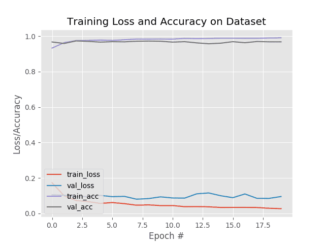
Our training loss decreases at a much sharper rate than our validation loss; furthermore, it appears that validation loss may be rising toward the end of training, indicating that the model may be overfitting.

Future experiments should look into applying additional regularization to the model as well as gathering additional training data.

In two weeks, I’ll show you how to take this fine-tuned ResNet model and use it in a practical, real-world application!

Stay tuned for the post; you won’t want to miss it!

Credits

This tutorial would not be possible without:

• Victor Gevers of the GDI.Foundation, who brought this project to my attention
• Nitin Rai who curated the normal clothes vs. camouflage clothes and posted the dataset on Kaggle
• Julia Riede who curated a variation of the dataset

Additionally, I’d like to credit Han et al. for the ResNet-152 visualization used in the header of this image.

Summary

In this tutorial you learned how to fine-tune ResNet with Keras and TensorFlow.

Fine-tuning is the process of:

1. Taking a pre-trained deep neural network (in this case, ResNet)
2. Removing the fully-connected layer head from the network
3. Placing a new, freshly initialized layer head on top of the body of the network
4. Optionally freezing the weights for the layers in the body
5. Training the model, using the pre-trained weights as a starting point to help the model learn faster

Using fine-tune we can obtain a higher accuracy model, typically with much less effort, data, and training time.

As a practical application, we fine-tuned ResNet on a dataset of camouflage vs. noncamouflage clothes images.

This dataset was curated and put together for us by PyImageSearch readers, Julia Riede and Nitin Rai — without them, this tutorial, as well as the project Victor Gevers and I were working on, would not have been possible! Please thank both Julia and Nitin if you see them online.

In two weeks, I’ll go into the details of the project that Victor Gevers and I have been working on, which wraps a nice a little bow on the following topics that we’ve recently covered on PyImageSearch:

• Face detection
• Age detection
• Removing duplicates from a deep learning dataset
• Fine-tuning a model for camouflage clothes vs. noncamouflage clothes detection

It’s a great post with very real applications to make the world a better place with computer vision and deep learning — you won’t want to miss it!

To download the source code to this post (and be notified when future tutorials are published here on PyImageSearch), simply enter your email address in the form below!