Whether you’re interested in learning how to apply facial recognition to video streams, building a complete deep learning pipeline for image classification, or simply want to tinker with your Raspberry Pi and add image recognition to a hobby project, you’ll need to learn OpenCV somewhere along the way.
A diverse dataset of images can greatly aid in learning OpenCV. Various image manipulations and processing techniques can be practiced and better understood with a wide range of images.
Roboflow has free tools for each stage of the computer vision pipeline that will streamline your workflows and supercharge your productivity.
Sign up or Log in to your Roboflow account to access state of the art dataset libaries and revolutionize your computer vision pipeline.
You can start by choosing your own datasets or using our PyimageSearch’s assorted library of useful datasets.
Bring data in any of 40+ formats to Roboflow, train using any state-of-the-art model architectures, deploy across multiple platforms (API, NVIDIA, browser, iOS, etc), and connect to applications or 3rd party tools.
The truth is that learning OpenCV used to be quite challenging. The documentation was hard to navigate. The tutorials were hard to follow and incomplete. And even some of the books were a bit tedious to work through.
The good news is learning OpenCV isn’t as hard as it used to be. And in fact, I’ll go as far as to say studying OpenCV has become significantly easier.
And to prove it to you (and help you learn OpenCV), I’ve put together this complete guide to learning the fundamentals of the OpenCV library using the Python programming language.
Let’s go ahead and get started learning the basics of OpenCV and image processing. By the end of today’s blog post, you’ll understand the fundamentals of OpenCV.
OpenCV Tutorial: A Guide to Learn OpenCV
This OpenCV tutorial is for beginners just getting started learning the basics. Inside this guide, you’ll learn basic image processing operations using the OpenCV library using Python.
And by the end of the tutorial you’ll be putting together a complete project to count basic objects in images using contours.
While this tutorial is aimed at beginners just getting started with image processing and the OpenCV library, I encourage you to give it a read even if you have a bit of experience.
A quick refresher in OpenCV basics will help you with your own projects as well.
Installing OpenCV and imutils on your system
The first step today is to install OpenCV on your system (if you haven’t already).
I maintain an OpenCV Install Tutorials page which contains links to previous OpenCV installation guides for Ubuntu, macOS, and Raspberry Pi.
You should visit that page and find + follow the appropriate guide for your system.
Once your fresh OpenCV development environment is set up, install the imutils package via pip. I have created and maintained imutils (source on GitHub) for the image processing community and it is used heavily on my blog. You should install imutils in the same environment you installed OpenCV into — you’ll need it to work through this blog post as it will facilitate basic image processing operations:
$ pip install imutils
Note: If you are using Python virtual environments don’t forget to use the workon command to enter your environment before installing imutils !
OpenCV Project Structure
Before going too far down the rabbit hole, be sure to grab the code + images from the “Downloads” section of today’s blog post.
From there, navigate to where you downloaded the .zip in your terminal (cd ). And then we can unzip the archive, change working directories (cd ) into the project folder, and analyze the project structure via tree :
$ cd ~/Downloads
$ unzip opencv-tutorial.zip
$ cd opencv-tutorial
$ tree
.
├── jp.png
├── opencv_tutorial_01.py
├── opencv_tutorial_02.py
└── tetris_blocks.png

0 directories, 4 files
In this tutorial we’ll be creating two Python scripts to help you learn OpenCV basics:
- Our first script,
opencv_tutorial_01.pywill cover basic image processing operations using an image from the movie, Jurassic Park (jp.png). - From there,
opencv_tutorial_02.pywill show you how to use these image processing building blocks to create an OpenCV application to count the number of objects in a Tetris image (tetris_blocks.png).
Loading and displaying an image
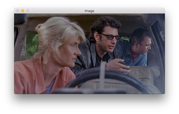
Let’s begin by opening up opencv_tutorial_01.py in your favorite text editor or IDE:
# import the necessary packages
import imutils
import cv2

# load the input image and show its dimensions, keeping in mind that
# images are represented as a multi-dimensional NumPy array with
# shape no. rows (height) x no. columns (width) x no. channels (depth)
image = cv2.imread("jp.png")
(h, w, d) = image.shape
print("width={}, height={}, depth={}".format(w, h, d))

# display the image to our screen -- we will need to click the window
# open by OpenCV and press a key on our keyboard to continue execution
cv2.imshow("Image", image)
cv2.waitKey(0)
On Lines 2 and 3 we import both imutils and cv2 . The cv2 package is OpenCV and despite the 2 embedded, it can actually be OpenCV 3 (or possibly OpenCV 4 which may be released later in 2018). The imutils package is my series of convenience functions.
Now that we have the required software at our fingertips via imports, let’s load an image from disk into memory.
To load our Jurassic Park image (from one of my favorite movies), we call cv2.imread("jp.png") . As you can see on Line 8, we assign the result to image . Our image is actually just a NumPy array.
Later in this script, we’ll need the height and width. So on Line 9, I call image.shape to extract the height, width, and depth.
It may seem confusing that the height comes before the width, but think of it this way:
- We describe matrices by # of rows x # of columns
- The number of rows is our height
- And the number of columns is our width
Therefore, the dimensions of an image represented as a NumPy array are actually represented as (height, width, depth).
Depth is the number of channels — in our case this is three since we’re working with 3 color channels: Blue, Green, and Red.
The print command shown on Line 10 will output the values to the terminal:
width=600, height=322, depth=3
To display the image on the screen using OpenCV we employ cv2.imshow("Image", image) on Line 14. The subsequent line waits for a keypress (Line 15). This is important otherwise our image would display and disappear faster than we’d even see the image.
Note: You need to actually click the active window opened by OpenCV and press a key on your keyboard to advance the script. OpenCV cannot monitor your terminal for input so if you a press a key in the terminal OpenCV will not notice. Again, you will need to click the active OpenCV window on your screen and press a key on your keyboard.
Accessing individual pixels
First, you may ask:
What is a pixel?
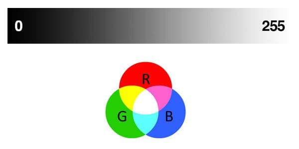
All images consist of pixels which are the raw building blocks of images. Images are made of pixels in a grid. A 640 x 480 image has 640 columns (the width) and 480 rows (the height). There are 640 * 480 = 307200 pixels in an image with those dimensions.
Each pixel in a grayscale image has a value representing the shade of gray. In OpenCV, there are 256 shades of gray — from 0 to 255. So a grayscale image would have a grayscale value associated with each pixel.
Pixels in a color image have additional information. There are several color spaces that you’ll soon become familiar with as you learn about image processing. For simplicity let’s only consider the RGB color space.
In OpenCV color images in the RGB (Red, Green, Blue) color space have a 3-tuple associated with each pixel: (B, G, R) .
Notice the ordering is BGR rather than RGB. This is because when OpenCV was first being developed many years ago the standard was BGR ordering. Over the years, the standard has now become RGB but OpenCV still maintains this “legacy” BGR ordering to ensure no existing code breaks.
Each value in the BGR 3-tuple has a range of [0, 255] . How many color possibilities are there for each pixel in an RGB image in OpenCV? That’s easy: 256 * 256 * 256 = 16777216 .
Now that we know exactly what a pixel is, let’s see how to retrieve the value of an individual pixel in the image:
# access the RGB pixel located at x=50, y=100, keepind in mind that
# OpenCV stores images in BGR order rather than RGB
(B, G, R) = image[100, 50]
print("R={}, G={}, B={}".format(R, G, B))
As shown previously, our image dimensions are width=600, height=322, depth=3 . We can access individual pixel values in the array by specifying the coordinates so long as they are within the max width and height.
The code, image[100, 50] , yields a 3-tuple of BGR values from the pixel located at x=50 and y=100 (again, keep in mind that the height is the number of rows and the width is the number of columns — take a second now to convince yourself this is true). As stated above, OpenCV stores images in BGR ordering (unlike Matplotlib, for example). Check out how simple it is to extract the color channel values for the pixel on Line 19.
The resulting pixel value is shown on the terminal here:
R=41, G=49, B=37
Array slicing and cropping
Extracting “regions of interest” (ROIs) is an important skill for image processing.
Say, for example, you’re working on recognizing faces in a movie. First, you’d run a face detection algorithm to find the coordinates of faces in all the frames you’re working with. Then you’d want to extract the face ROIs and either save them or process them. Locating all frames containing Dr. Ian Malcolm in Jurassic Park would be a great face recognition mini-project to work on.
For now, let’s just manually extract an ROI. This can be accomplished with array slicing.
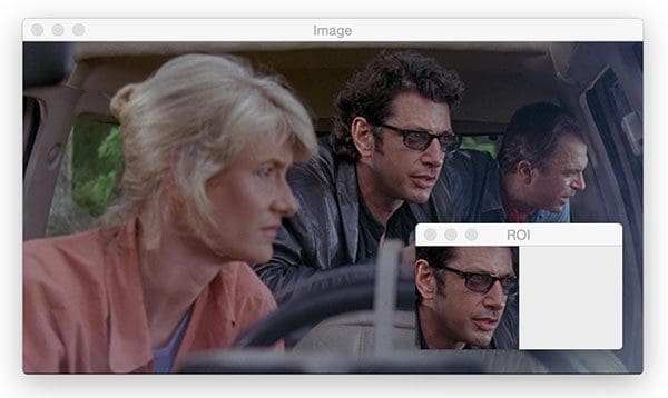
# extract a 100x100 pixel square ROI (Region of Interest) from the
# input image starting at x=320,y=60 at ending at x=420,y=160
roi = image[60:160, 320:420]
cv2.imshow("ROI", roi)
cv2.waitKey(0)
Array slicing is shown on Line 24 with the format: image[startY:endY, startX:endX] . This code grabs an roi which we then display on Line 25. Just like last time, we display until a key is pressed (Line 26).
As you can see in Figure 3, we’ve extracted the face of Dr. Ian Malcolm. I actually predetermined the (x, y)-coordinates using Photoshop for this example, but if you stick with me on the blog you could detect and extract face ROI’s automatically.
Resizing images
Resizing images is important for a number of reasons. First, you might want to resize a large image to fit on your screen. Image processing is also faster on smaller images because there are fewer pixels to process. In the case of deep learning, we often resize images, ignoring aspect ratio, so that the volume fits into a network which requires that an image be square and of a certain dimension.
Let’s resize our original image to 200 x 200 pixels:
# resize the image to 200x200px, ignoring aspect ratio
resized = cv2.resize(image, (200, 200))
cv2.imshow("Fixed Resizing", resized)
cv2.waitKey(0)
On Line 29, we have resized an image ignoring aspect ratio. Figure 4 (right) shows that the image is resized but is now distorted because we didn’t take into account the aspect ratio.
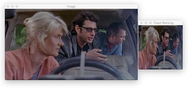
cv2.resize however aspect ratio is not preserved automatically.Let’s calculate the aspect ratio of the original image and use it to resize an image so that it doesn’t appear squished and distorted:
# fixed resizing and distort aspect ratio so let's resize the width
# to be 300px but compute the new height based on the aspect ratio
r = 300.0 / w
dim = (300, int(h * r))
resized = cv2.resize(image, dim)
cv2.imshow("Aspect Ratio Resize", resized)
cv2.waitKey(0)
Recall back to Line 9 of this script where we extracted the width and height of the image.
Let’s say that we want to take our 600-pixel wide image and resize it to 300 pixels wide while maintaining aspect ratio.
On Line 35 we calculate the ratio of the new width to the old width (which happens to be 0.5).
From there, we specify our dimensions of the new image, dim . We know that we want a 300-pixel wide image, but we must calculate the height using the ratio by multiplying h by r (the original height and our ratio respectively).
Feeding dim (our dimensions) into the cv2.resize function, we’ve now obtained a new image named resized which is not distorted (Line 37).
To check our work, we display the image using the code on Line 38:
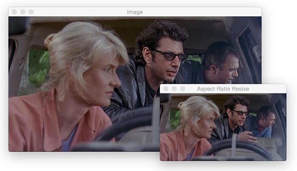
cv2.resize) along one dimension and multiply the other dimension by the aspect ratio. See Figure 6 for an even easier method.But can we make this process of preserving aspect ratio during resizing even easier?
Yes!
Computing the aspect ratio each time we want to resize an image is a bit tedious, so I wrapped the code in a function within imutils .
Here is how you may use imutils.resize :
# manually computing the aspect ratio can be a pain so let's use the
# imutils library instead
resized = imutils.resize(image, width=300)
cv2.imshow("Imutils Resize", resized)
cv2.waitKey(0)
In a single line of code, we’ve preserved aspect ratio and resized the image.
Simple right?
All you need to provide is your target width or target height as a keyword argument (Line 43).
Here’s the result:
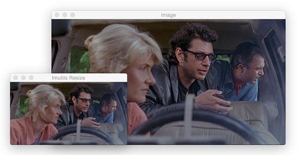
imutils.resize. Now your image won’t risk being “squished” as in Figure 4.Rotating an image
Let’s rotate our Jurassic Park image for our next example:
# let's rotate an image 45 degrees clockwise using OpenCV by first
# computing the image center, then constructing the rotation matrix,
# and then finally applying the affine warp
center = (w // 2, h // 2)
M = cv2.getRotationMatrix2D(center, -45, 1.0)
rotated = cv2.warpAffine(image, M, (w, h))
cv2.imshow("OpenCV Rotation", rotated)
cv2.waitKey(0)
Rotating an image about the center point requires that we first calculate the center (x, y)-coordinates of the image (Line 50).
Note: We use // to perform integer math (i.e., no floating point values).
From there we calculate a rotation matrix, M (Line 51). The -45 means that we’ll rotate the image 45 degrees clockwise. Recall from your middle/high school geometry class about the unit circle and you’ll be able to remind yourself that positive angles are counterclockwise and negative angles are clockwise.
From there we warp the image using the matrix (effectively rotating it) on Line 52.
The rotated image is displayed to the screen on Line 52 and is shown in Figure 7:
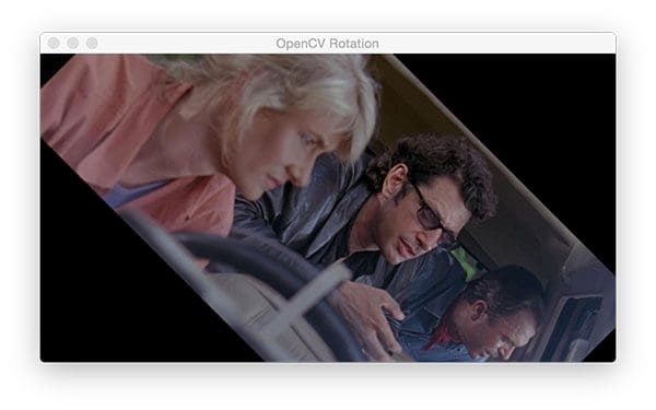
cv2.getRotationMatrix2D, and (3) use the rotation matrix to warp the image with cv2.warpAffine.Now let’s perform the same operation in just a single line of code using imutils :
# rotation can also be easily accomplished via imutils with less code
rotated = imutils.rotate(image, -45)
cv2.imshow("Imutils Rotation", rotated)
cv2.waitKey(0)
Since I don’t have to rotate image as much as resizing them (comparatively) I find the rotation process harder to remember. Therefore, I created a function in imutils to handle it for us. In a single line of code, I can accomplish rotating the image 45 degrees clockwise (Line 57) as in Figure 8:

imutils.rotate, we can rotate an image with OpenCV and Python conveniently with a single line of code.At this point you have to be thinking:
Why in the world is the image clipped?
The thing is, OpenCV doesn’t care if our image is clipped and out of view after the rotation. I find this to be quite bothersome, so here’s my imutils version which will keep the entire image in view. I call it rotate_bound :
# OpenCV doesn't "care" if our rotated image is clipped after rotation
# so we can instead use another imutils convenience function to help
# us out
rotated = imutils.rotate_bound(image, 45)
cv2.imshow("Imutils Bound Rotation", rotated)
cv2.waitKey(0)
There’s a lot going on behind the scenes of rotate_bound . If you’re interested in how the method on Line 64 works, be sure to check out this blog post.
The result is shown in Figure 9:
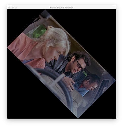
rotate_bound function of imutils will prevent OpenCV from clipping the image during a rotation. See this blog post to learn how it works!Perfect! The entire image is in the frame and it is correctly rotated 45 degrees clockwise.
Smoothing an image
In many image processing pipelines, we must blur an image to reduce high-frequency noise, making it easier for our algorithms to detect and understand the actual contents of the image rather than just noise that will “confuse” our algorithms. Blurring an image is very easy in OpenCV and there are a number of ways to accomplish it.
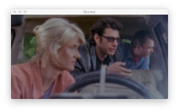
11 x 11 kernel using OpenCV. Blurring is an important step of many image processing pipelines to reduce high-frequency noise.I often use the GaussianBlur function:
# apply a Gaussian blur with a 11x11 kernel to the image to smooth it,
# useful when reducing high frequency noise
blurred = cv2.GaussianBlur(image, (11, 11), 0)
cv2.imshow("Blurred", blurred)
cv2.waitKey(0)
On Line 70 we perform a Gaussian Blur with an 11 x 11 kernel the result of which is shown in Figure 10.
Larger kernels would yield a more blurry image. Smaller kernels will create less blurry images. To read more about kernels, refer to this blog post or the PyImageSearch Gurus course.
Drawing on an image
In this section, we’re going to draw a rectangle, circle, and line on an input image. We’ll also overlay text on an image as well.
Before we move on with drawing on an image with OpenCV, take note that drawing operations on images are performed in-place. Therefore at the beginning of each code block, we make a copy of the original image storing the copy as output . We then proceed to draw on the image called output in-place so we do not destroy our original image.
Let’s draw a rectangle around Ian Malcolm’s face:
# draw a 2px thick red rectangle surrounding the face
output = image.copy()
cv2.rectangle(output, (320, 60), (420, 160), (0, 0, 255), 2)
cv2.imshow("Rectangle", output)
cv2.waitKey(0)
First, we make a copy of the image on Line 75 for reasons just explained.
Then we proceed to draw the rectangle.
Drawing rectangles in OpenCV couldn’t be any easier. Using pre-calculated coordinates, I’ve supplied the following parameters to the cv2.rectangle function on Line 76:
img: The destination image to draw upon. We’re drawing onoutput.pt1: Our starting pixel coordinate which is the top-left. In our case, the top-left is(320, 60).pt2: The ending pixel — bottom-right. The bottom-right pixel is located at(420, 160).color: BGR tuple. To represent red, I’ve supplied(0 , 0, 255).thickness: Line thickness (a negative value will make a solid rectangle). I’ve supplied a thickness of2.
Since we are using OpenCV’s functions rather than NumPy operations we can supply our coordinates in (x, y) order rather than (y, x) since we are not manipulating or accessing the NumPy array directly — OpenCV is taking care of that for us.
Here’s our result in Figure 11:

cv2.rectangle. I pre-determined the coordinates around the face for this example, but you could use a face detection method to automatically find the face coordinates.And now let’s place a solid blue circle in front of Dr. Ellie Sattler’s face:
# draw a blue 20px (filled in) circle on the image centered at
# x=300,y=150
output = image.copy()
cv2.circle(output, (300, 150), 20, (255, 0, 0), -1)
cv2.imshow("Circle", output)
cv2.waitKey(0)
To draw a circle, you need to supply following parameters to cv2.circle :
img: The output image.center: Our circle’s center coordinate. I supplied(300, 150)which is right in front of Ellie’s eyes.radius: The circle radius in pixels. I provided a value of20pixels.color: Circle color. This time I went with blue as is denoted by 255 in the B and 0s in the G + R components of the BGR tuple,(255, 0, 0).thickness: The line thickness. Since I supplied a negative value (-1), the circle is solid/filled in.
Here’s the result in Figure 12:
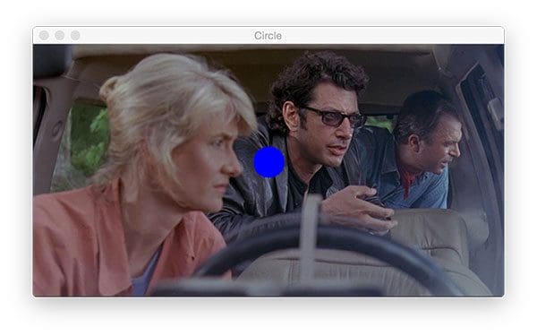
cv2.circle method allows you to draw circles anywhere on an image. I’ve drawn a solid circle for this example as is denoted by the -1 line thickness parameter (positive values will make a circular outline with variable line thickness).It looks like Ellie is more interested in the dinosaurs than my big blue dot, so let’s move on!
Next, we’ll draw a red line. This line goes through Ellie’s head, past her eye, and to Ian’s hand.
If you look carefully at the method parameters and compare them to that of the rectangle, you’ll notice that they are identical:
# draw a 5px thick red line from x=60,y=20 to x=400,y=200
output = image.copy()
cv2.line(output, (60, 20), (400, 200), (0, 0, 255), 5)
cv2.imshow("Line", output)
cv2.waitKey(0)
Just as in a rectangle, we supply two points, a color, and a line thickness. OpenCV’s backend does the rest.
Figure 13 shows the result of Line 89 from the code block:
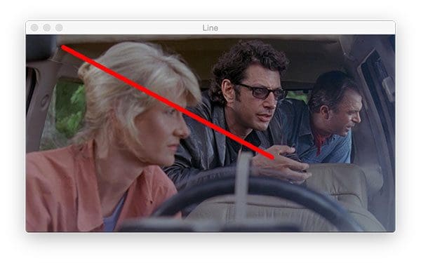
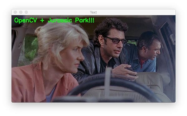
cv2.line only requires a starting point, ending point, color, and thickness.Oftentimes you’ll find that you want to overlay text on an image for display purposes. If you’re working on face recognition you’ll likely want to draw the person’s name above their face. Or if you advance in your computer vision career you may build an image classifier or object detector. In these cases, you’ll find that you want to draw text containing the class name and probability.
Let’s see how OpenCV’s putText function works:
# draw green text on the image
output = image.copy()
cv2.putText(output, "OpenCV + Jurassic Park!!!", (10, 25),
	cv2.FONT_HERSHEY_SIMPLEX, 0.7, (0, 255, 0), 2)
cv2.imshow("Text", output)
cv2.waitKey(0)
The putText function of OpenCV is responsible for drawing text on an image. Let’s take a look at the required parameters:
img: The output image.text: The string of text we’d like to write/draw on the image.pt: The starting point for the text.font: I often use thecv2.FONT_HERSHEY_SIMPLEX. The available fonts are listed here.scale: Font size multiplier.color: Text color.thickness: The thickness of the stroke in pixels.
The code on Lines 95 and 96 will draw the text, “OpenCV + Jurassic Park!!!” in green on our output image in Figure 14:
cv2.putText code shown above you can practice overlaying text on an image with different colors, fonts, sizes, and/or locations.Running the first OpenCV tutorial Python script
In my blog posts, I generally provide a section detailing how you can run the code on your computer. At this point in the blog post, I make the following assumptions:
- You have downloaded the code from the “Downloads” section of this blog post.
- You have unzipped the files.
- You have installed OpenCV and the imutils library on your system.
To execute our first script, open a terminal or command window and navigate to the files or extract them if necessary.
From there, enter the following command:
$ python opencv_tutorial_01.py
width=600, height=322, depth=3
R=41, G=49, B=37
The command is everything after the bash prompt $ character. Just type python opencv_tutorial_01.py in your terminal and then the first image will appear.
To cycle through each step that we just learned, make sure an image window is active, and press any key.
Our first couple code blocks above told Python to print information in the terminal. If your terminal is visible, you’ll see the terminal output (Lines 2 and 3) shown.
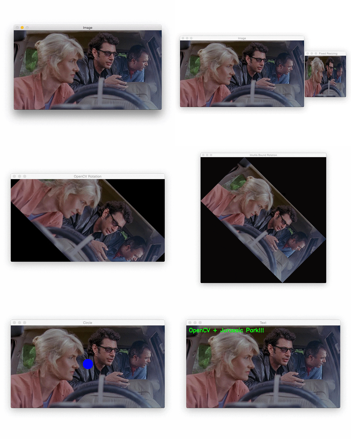
I’ve also included a GIF animation demonstrating all the image processing steps we took sequentially, one right after the other:
Counting objects
Now we’re going to shift gears and work on the second script included in the “Downloads” associated with this blog post.
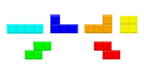
In the next few sections we’ll learn how to use create a simple Python + OpenCV script to count the number of Tetris blocks in the following image:
Along the way we’ll be:
- Learning how to convert images to grayscale with OpenCV
- Performing edge detection
- Thresholding a grayscale image
- Finding, counting, and drawing contours
- Conducting erosion and dilation
- Masking an image
Go ahead and close the first script you downloaded and open up opencv_tutorial_02.py to get started with the second example:
# import the necessary packages
import argparse
import imutils
import cv2

# construct the argument parser and parse the arguments
ap = argparse.ArgumentParser()
ap.add_argument("-i", "--image", required=True,
	help="path to input image")
args = vars(ap.parse_args())
On Lines 2-4 we import our packages. This is necessary at the start of each Python script. For this second script, I’ve imported argparse — a command line arguments parsing package which comes with all installations of Python.
Take a quick glance at Lines 7-10. These lines allow us to provide additional information to our program at runtime from within the terminal. Command line arguments are used heavily on the PyImageSearch blog and in all other computer science fields as well.
I encourage you to read about them on this post: Python, argparse, and command line arguments.
We have one required command line argument --image , as is defined on Lines 8 and 9.
We’ll learn how to run the script with the required command line argument down below. For now, just know that wherever you encounter args["image"] in the script, we’re referring to the path to the input image.
Converting an image to grayscale
# load the input image (whose path was supplied via command line
# argument) and display the image to our screen
image = cv2.imread(args["image"])
cv2.imshow("Image", image)
cv2.waitKey(0)

# convert the image to grayscale
gray = cv2.cvtColor(image, cv2.COLOR_BGR2GRAY)
cv2.imshow("Gray", gray)
cv2.waitKey(0)
We load the image into memory on Line 14. The parameter to the cv2.imread function is our path contained in the args dictionary referenced with the "image" key, args["image"] .
From there, we display the image until we encounter our first keypress (Lines 15 and 16).
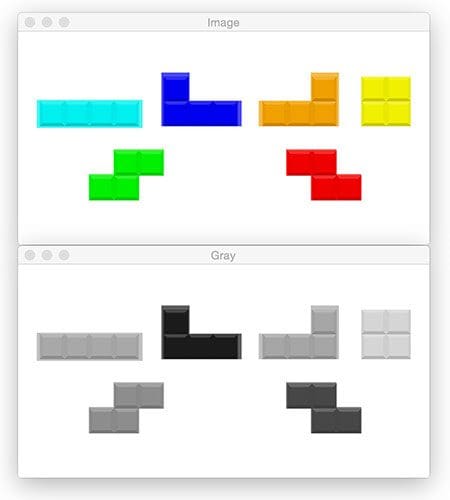
We’re going to be thresholding and detecting edges in the image shortly. Therefore we convert the image to grayscale on Line 19 by calling cv2.cvtColor and providing the image and cv2.COLOR_BGR2GRAY flag.
Again we display the image and wait for a keypress (Lines 20 and 21).
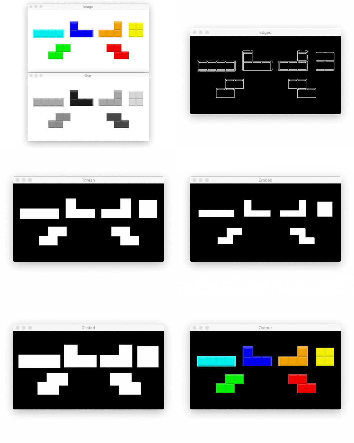
The result of our conversion to grayscale is shown in Figure 17 (bottom).
Edge detection
Edge detection is useful for finding boundaries of objects in an image — it is effective for segmentation purposes.
Let’s perform edge detection to see how the process works:
# applying edge detection we can find the outlines of objects in
# images
edged = cv2.Canny(gray, 30, 150)
cv2.imshow("Edged", edged)
cv2.waitKey(0)
Using the popular Canny algorithm (developed by John F. Canny in 1986), we can find the edges in the image.
We provide three parameters to the cv2.Canny function:
img: Thegrayimage.minVal: A minimum threshold, in our case30.maxVal: The maximum threshold which is150in our example.aperture_size: The Sobel kernel size. By default this value is3and hence is not shown on Line 25.
Different values for the minimum and maximum thresholds will return different edge maps.
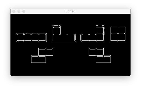
In Figure 18 below, notice how edges of Tetris blocks themselves are revealed along with sub-blocks that make up the Tetris block:
Thresholding
Image thresholding is an important intermediary step for image processing pipelines. Thresholding can help us to remove lighter or darker regions and contours of images.
I highly encourage you to experiment with thresholding. I tuned the following code to work for our example by trial and error (as well as experience):
# threshold the image by setting all pixel values less than 225
# to 255 (white; foreground) and all pixel values >= 225 to 255
# (black; background), thereby segmenting the image
thresh = cv2.threshold(gray, 225, 255, cv2.THRESH_BINARY_INV)[1]
cv2.imshow("Thresh", thresh)
cv2.waitKey(0)
In a single line (Line 32) we are:
- Grabbing all pixels in the
grayimage greater than 225 and setting them to 0 (black) which corresponds to the background of the image - Setting pixel vales less than 225 to 255 (white) which corresponds to the foreground of the image (i.e., the Tetris blocks themselves).
For more information on the cv2.threshold function, including how the thresholding flags work, be sure to refer to official OpenCV documentation.
Segmenting foreground from background with a binary image is critical to finding contours (our next step).
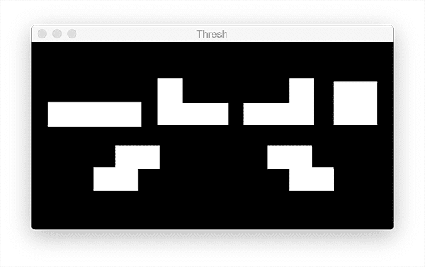
Notice in Figure 19 that the foreground objects are white and the background is black.
Detecting and drawing contours
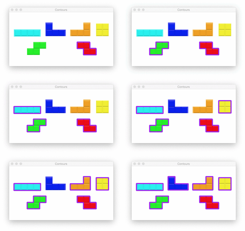
Pictured in the Figure 20 animation, we have 6 shape contours. Let’s find and draw their outlines via code:
# find contours (i.e., outlines) of the foreground objects in the
# thresholded image
cnts = cv2.findContours(thresh.copy(), cv2.RETR_EXTERNAL,
	cv2.CHAIN_APPROX_SIMPLE)
cnts = imutils.grab_contours(cnts)
output = image.copy()

# loop over the contours
for c in cnts:
	# draw each contour on the output image with a 3px thick purple
	# outline, then display the output contours one at a time
	cv2.drawContours(output, [c], -1, (240, 0, 159), 3)
	cv2.imshow("Contours", output)
	cv2.waitKey(0)
On Lines 38 and 39, we use cv2.findContours to detect the contours in the image. Take note of the parameter flags but for now let’s keep things simple — our algorithm is finding all foreground (white) pixels in the thresh.copy() image.
Line 40 is very important accounting for the fact that cv2.findContours implementation changed between OpenCV 2.4, OpenCV 3, and OpenCV 4. This compatibility line is present on the blog wherever contours are involved.
We make a copy of the original image on Line 41 so that we can draw contours on subsequent Lines 44-49.
On Line 47 we draw each c from the cnts list on the image using the appropriately named cv2.drawContours . I chose purple which is represented by the tuple (240, 0, 159) .
Using what we learned earlier in this blog post, let’s overlay some text on the image:
# draw the total number of contours found in purple
text = "I found {} objects!".format(len(cnts))
cv2.putText(output, text, (10, 25),  cv2.FONT_HERSHEY_SIMPLEX, 0.7,
	(240, 0, 159), 2)
cv2.imshow("Contours", output)
cv2.waitKey(0)
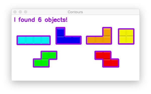
Line 52 builds a text string containing the number of shape contours. Counting the total number of objects in this image is as simple as checking the length of the contours list — len(cnts) .
The result is shown in Figure 21:
len(cnts).Erosions and dilations
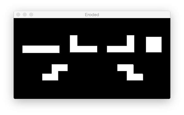
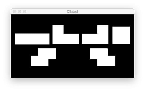
Erosions and dilations are typically used to reduce noise in binary images (a side effect of thresholding).
To reduce the size of foreground objects we can erode away pixels given a number of iterations:
# we apply erosions to reduce the size of foreground objects
mask = thresh.copy()
mask = cv2.erode(mask, None, iterations=5)
cv2.imshow("Eroded", mask)
cv2.waitKey(0)
On Line 59 we copy the thresh image while naming it mask .
Then, utilizing cv2.erode , we proceed to reduce the contour sizes with 5 iterations (Line 60).
Demonstrated in Figure 22, the masks generated from the Tetris contours are slightly smaller:
Similarly, we can foreground regions in the mask. To enlarge the regions, simply use cv2.dilate :
# similarly, dilations can increase the size of the ground objects
mask = thresh.copy()
mask = cv2.dilate(mask, None, iterations=5)
cv2.imshow("Dilated", mask)
cv2.waitKey(0)
Masking and bitwise operations
Masks allow us to “mask out” regions of an image we are uninterested in. We call them “masks” because they will hide regions of images we do not care about.
If we use the thresh image from Figure 18 and mask it with the original image, we’re presented with Figure 23:
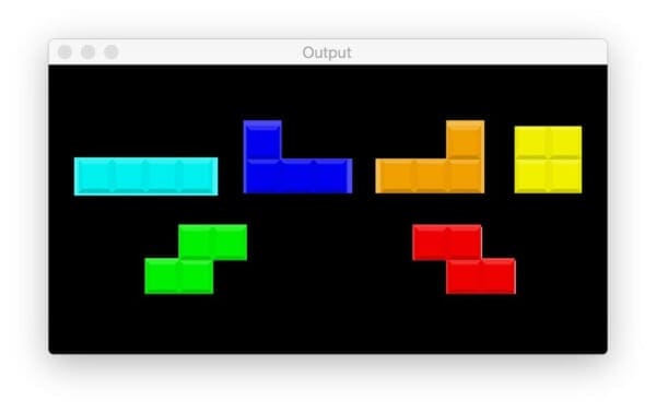
In Figure 24, the background is black now and our foreground consists of colored pixels — any pixels masked by our mask image.
Let’s learn how to accomplish this:
# a typical operation we may want to apply is to take our mask and
# apply a bitwise AND to our input image, keeping only the masked
# regions
mask = thresh.copy()
output = cv2.bitwise_and(image, image, mask=mask)
cv2.imshow("Output", output)
cv2.waitKey(0)
The mask is generated by copying the binary thresh image (Line 73).
From there we bitwise AND the pixels from both images together using cv2.bitwise_and .
The result is Figure 24 above where now we’re only showing/highlighting the Tetris blocks.
Running the second OpenCV tutorial Python script
To run the second script, be sure you’re in the folder containing your downloaded source code and Python scripts. From there, we’ll open up a terminal provide the script name + command line argument:
$ python opencv_tutorial_02.py --image tetris_blocks.png
The argument flag is --image and the image argument itself is tetris_blocks.png — a path to the relevant file in the directory.
There is no terminal output for this script. Again, to cycle through the images, be sure you click on an image window to make it active, from there you can press a key and it will be captured to move forward to the next waitKey(0) in the script. When the program is finished running, your script will exit gracefully and you’ll be presented with a new bash prompt line in your terminal.
Below I have included a GIF animation of the basic OpenCV image processing steps in our example script:
What's next? We recommend PyImageSearch University.
86+ total classes • 115+ hours hours of on-demand code walkthrough videos • Last updated: May 2026
★★★★★ 4.84 (128 Ratings) • 16,000+ Students Enrolled
I strongly believe that if you had the right teacher you could master computer vision and deep learning.
Do you think learning computer vision and deep learning has to be time-consuming, overwhelming, and complicated? Or has to involve complex mathematics and equations? Or requires a degree in computer science?
That’s not the case.
All you need to master computer vision and deep learning is for someone to explain things to you in simple, intuitive terms. And that’s exactly what I do. My mission is to change education and how complex Artificial Intelligence topics are taught.
If you're serious about learning computer vision, your next stop should be PyImageSearch University, the most comprehensive computer vision, deep learning, and OpenCV course online today. Here you’ll learn how to successfully and confidently apply computer vision to your work, research, and projects. Join me in computer vision mastery.
Inside PyImageSearch University you'll find:
- ✓ 86+ courses on essential computer vision, deep learning, and OpenCV topics
- ✓ 86 Certificates of Completion
- ✓ 115+ hours hours of on-demand video
- ✓ Brand new courses released regularly, ensuring you can keep up with state-of-the-art techniques
- ✓ Pre-configured Jupyter Notebooks in Google Colab
- ✓ Run all code examples in your web browser — works on Windows, macOS, and Linux (no dev environment configuration required!)
- ✓ Access to centralized code repos for all 540+ tutorials on PyImageSearch
- ✓ Easy one-click downloads for code, datasets, pre-trained models, etc.
- ✓ Access on mobile, laptop, desktop, etc.
Summary
In today’s blog post you learned the fundamentals of image processing and OpenCV using the Python programming language.
You are now prepared to start using these image processing operations as “building blocks” you can chain together to build an actual computer vision application — a great example of such a project is the basic object counter we created by counting contours.
I hope this tutorial helped you learn OpenCV!
To be notified when future OpenCV blog posts are published here on PyImageSearch, just enter your email address in the form below!

Download the Source Code and FREE 17-page Resource Guide
Enter your email address below to get a .zip of the code and a FREE 17-page Resource Guide on Computer Vision, OpenCV, and Deep Learning. Inside you'll find my hand-picked tutorials, books, courses, and libraries to help you master CV and DL!
