Last Updated on July 1, 2021
Would you have guessed that I’m a stamp collector?
Just kidding. I’m not.
But let’s play a little game of pretend.
Let’s pretend that we have a huge dataset of stamp images. And we want to take two arbitrary stamp images and compare them to determine if they are identical, or near identical in some way.
In general, we can accomplish this in two ways.
The first method is to use locality sensitive hashing, which I’ll cover in a later blog post.
The second method is to use algorithms such as Mean Squared Error (MSE) or the Structural Similarity Index (SSIM).
In this blog post I’ll show you how to use Python to compare two images using Mean Squared Error and Structural Similarity Index.
- Update July 2021: Updated SSIM import from scikit-image per the latest API update. Added section on alternative image comparison methods, including resources on siamese networks.
Our Example Dataset
Let’s start off by taking a look at our example dataset:

Here you can see that we have three images: (left) our original image of our friends from Jurassic Park going on their first (and only) tour, (middle) the original image with contrast adjustments applied to it, and (right), the original image with the Jurassic Park logo overlaid on top of it via Photoshop manipulation.
Now, it’s clear to us that the left and the middle images are more “similar” to each other — the one in the middle is just like the first one, only it is “darker”.
But as we’ll find out, Mean Squared Error will actually say the Photoshopped image is more similar to the original than the middle image with contrast adjustments. Pretty weird, right?
Mean Squared Error vs. Structural Similarity Measure
Let’s take a look at the Mean Squared error equation:

While this equation may look complex, I promise you it’s not.
And to demonstrate this you, I’m going to convert this equation to a Python function:
def mse(imageA, imageB):
	# the 'Mean Squared Error' between the two images is the
	# sum of the squared difference between the two images;
	# NOTE: the two images must have the same dimension
	err = np.sum((imageA.astype("float") - imageB.astype("float")) ** 2)
	err /= float(imageA.shape[0] * imageA.shape[1])

	# return the MSE, the lower the error, the more "similar"
	# the two images are
	return err
So there you have it — Mean Squared Error in only four lines of Python code once you take out the comments.
Let’s tear it apart and see what’s going on:
- On Line 7 we define our
msefunction, which takes two arguments:imageAandimageB(i.e. the images we want to compare for similarity). - All the real work is handled on Line 11. First we convert the images from unsigned 8-bit integers to floating point, that way we don’t run into any problems with modulus operations “wrapping around”. We then take the difference between the images by subtracting the pixel intensities. Next up, we square these difference (hence mean squared error, and finally sum them up.
- Line 12 handles the mean of the Mean Squared Error. All we are doing is dividing our sum of squares by the total number of pixels in the image.
- Finally, we return our MSE to the caller one Line 16.
MSE is dead simple to implement — but when using it for similarity, we can run into problems. The main one being that large distances between pixel intensities do not necessarily mean the contents of the images are dramatically different. I’ll provide some proof for that statement later in this post, but in the meantime, take my word for it.
It’s important to note that a value of 0 for MSE indicates perfect similarity. A value greater than one implies less similarity and will continue to grow as the average difference between pixel intensities increases as well.
In order to remedy some of the issues associated with MSE for image comparison, we have the Structural Similarity Index, developed by Wang et al.:

The SSIM method is clearly more involved than the MSE method, but the gist is that SSIM attempts to model the perceived change in the structural information of the image, whereas MSE is actually estimating the perceived errors. There is a subtle difference between the two, but the results are dramatic.
Furthermore, the equation in Equation 2 is used to compare two windows (i.e. small sub-samples) rather than the entire image as in MSE. Doing this leads to a more robust approach that is able to account for changes in the structure of the image, rather than just the perceived change.
The parameters to Equation 2 include the (x, y) location of the N x N window in each image, the mean of the pixel intensities in the x and y direction, the variance of intensities in the x and y direction, along with the covariance.
Unlike MSE, the SSIM value can vary between -1 and 1, where 1 indicates perfect similarity.
Luckily, as you’ll see, we don’t have to implement this method by hand since scikit-image already has an implementation ready for us.
Let’s go ahead and jump into some code.
How-To: Compare Two Images Using Python
# import the necessary packages
from skimage.metrics import structural_similarity as ssim
import matplotlib.pyplot as plt
import numpy as np
import cv2
We start by importing the packages we’ll need — matplotlib for plotting, NumPy for numerical processing, and cv2 for our OpenCV bindings. Our Structural Similarity Index method is already implemented for us by scikit-image, so we’ll just use their implementation.
def mse(imageA, imageB):
	# the 'Mean Squared Error' between the two images is the
	# sum of the squared difference between the two images;
	# NOTE: the two images must have the same dimension
	err = np.sum((imageA.astype("float") - imageB.astype("float")) ** 2)
	err /= float(imageA.shape[0] * imageA.shape[1])

	# return the MSE, the lower the error, the more "similar"
	# the two images are
	return err

def compare_images(imageA, imageB, title):
	# compute the mean squared error and structural similarity
	# index for the images
	m = mse(imageA, imageB)
	s = ssim(imageA, imageB)

	# setup the figure
	fig = plt.figure(title)
	plt.suptitle("MSE: %.2f, SSIM: %.2f" % (m, s))

	# show first image
	ax = fig.add_subplot(1, 2, 1)
	plt.imshow(imageA, cmap = plt.cm.gray)
	plt.axis("off")

	# show the second image
	ax = fig.add_subplot(1, 2, 2)
	plt.imshow(imageB, cmap = plt.cm.gray)
	plt.axis("off")

	# show the images
	plt.show()
Lines 7-16 define our mse method, which you are already familiar with.
We then define the compare_images function on Line 18 which we’ll use to compare two images using both MSE and SSIM. The mse function takes three arguments: imageA and imageB, which are the two images we are going to compare, and then the title of our figure.
We then compute the MSE and SSIM between the two images on Lines 21 and 22.
Lines 25-39 handle some simple matplotlib plotting. We simply display the MSE and SSIM associated with the two images we are comparing.
# load the images -- the original, the original + contrast,
# and the original + photoshop
original = cv2.imread("images/jp_gates_original.png")
contrast = cv2.imread("images/jp_gates_contrast.png")
shopped = cv2.imread("images/jp_gates_photoshopped.png")

# convert the images to grayscale
original = cv2.cvtColor(original, cv2.COLOR_BGR2GRAY)
contrast = cv2.cvtColor(contrast, cv2.COLOR_BGR2GRAY)
shopped = cv2.cvtColor(shopped, cv2.COLOR_BGR2GRAY)
Lines 43-45 handle loading our images off disk using OpenCV. We’ll be using our original image (Line 43), our contrast adjusted image (Line 44), and our Photoshopped image with the Jurassic Park logo overlaid (Line 45).
We then convert our images to grayscale on Lines 48-50.
# initialize the figure
fig = plt.figure("Images")
images = ("Original", original), ("Contrast", contrast), ("Photoshopped", shopped)

# loop over the images
for (i, (name, image)) in enumerate(images):
	# show the image
	ax = fig.add_subplot(1, 3, i + 1)
	ax.set_title(name)
	plt.imshow(image, cmap = plt.cm.gray)
	plt.axis("off")

# show the figure
plt.show()

# compare the images
compare_images(original, original, "Original vs. Original")
compare_images(original, contrast, "Original vs. Contrast")
compare_images(original, shopped, "Original vs. Photoshopped")
Now that our images are loaded off disk, let’s show them. On Lines 52-65 we simply generate a matplotlib figure, loop over our images one-by-one, and add them to our plot. Our plot is then displayed to us on Line 65.
Finally, we can compare our images together using the compare_images function on Lines 68-70.
We can execute our script by issuing the following command:
$ python compare.py
Results
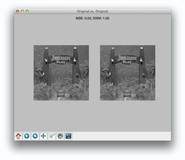
Once our script has executed, we should first see our test case — comparing the original image to itself:

Not surpassingly, the original image is identical to itself, with a value of 0.0 for MSE and 1.0 for SSIM. Remember, as the MSE increases the images are less similar, as opposed to the SSIM where smaller values indicate less similarity.
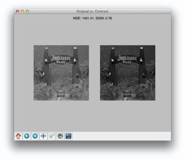
Now, take a look at comparing the original to the contrast adjusted image:

In this case, the MSE has increased and the SSIM decreased, implying that the images are less similar. This is indeed true — adjusting the contrast has definitely “damaged” the representation of the image.
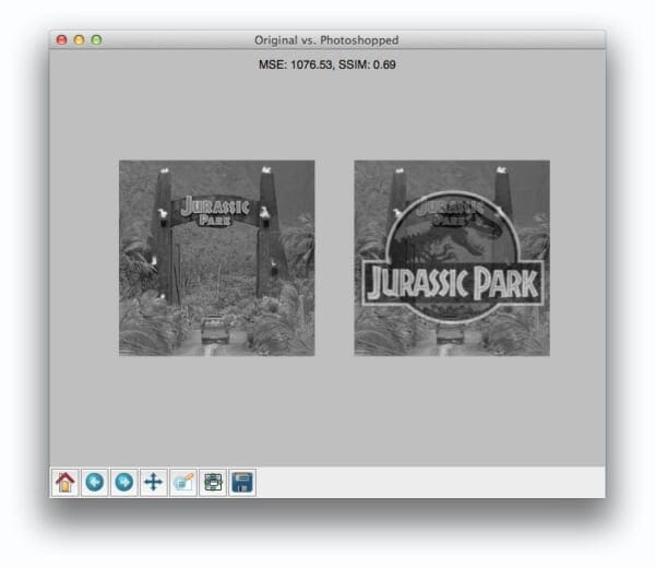
But things don’t get interesting until we compare the original image to the Photoshopped overlay:

Comparing the original image to the Photoshop overlay yields a MSE of 1076 and a SSIM of 0.69.
Wait a second.
A MSE of 1076 is smaller than the previous of 1401. But clearly the Photoshopped overlay is dramatically more different than simply adjusting the contrast! But again, this is a limitation we must accept when utilizing raw pixel intensities globally.
On the other end, SSIM is returns a value of 0.69, which is indeed less than the 0.78 obtained when comparing the original image to the contrast adjusted image.
Alternative Image Comparison Methods
MSE and SSIM are traditional computer vision and image processing methods to compare images. They tend to work best when images are near-perfectly aligned (otherwise, the pixel locations and values would not match up, throwing off the similarity score).
An alternative approach that works well when the two images are captured under different viewing angles, lighting conditions, etc., is to use keypoint detectors and local invariant descriptors, including SIFT, SURF, ORB, etc. This tutorial shows you how to implement RootSIFT, a more accurate variant of the popular SIFT detector and descriptor.
Furthermore, there are deep learning-based image similarity methods that we can utilize, particularly siamese networks. Siamese networks are super powerful models that can be trained with very little data to compute accurate image similarity scores.
The following tutorials will teach you about siamese networks:
- Building image pairs for siamese networks with Python
- Siamese networks with Keras, TensorFlow, and Deep Learning
- Comparing images for similarity using siamese networks, Keras, and TensorFlow
Additionally, siamese networks are covered in detail inside PyImageSearch University.
What's next? We recommend PyImageSearch University.
86+ total classes • 115+ hours hours of on-demand code walkthrough videos • Last updated: April 2026
★★★★★ 4.84 (128 Ratings) • 16,000+ Students Enrolled
I strongly believe that if you had the right teacher you could master computer vision and deep learning.
Do you think learning computer vision and deep learning has to be time-consuming, overwhelming, and complicated? Or has to involve complex mathematics and equations? Or requires a degree in computer science?
That’s not the case.
All you need to master computer vision and deep learning is for someone to explain things to you in simple, intuitive terms. And that’s exactly what I do. My mission is to change education and how complex Artificial Intelligence topics are taught.
If you're serious about learning computer vision, your next stop should be PyImageSearch University, the most comprehensive computer vision, deep learning, and OpenCV course online today. Here you’ll learn how to successfully and confidently apply computer vision to your work, research, and projects. Join me in computer vision mastery.
Inside PyImageSearch University you'll find:
- ✓ 86+ courses on essential computer vision, deep learning, and OpenCV topics
- ✓ 86 Certificates of Completion
- ✓ 115+ hours hours of on-demand video
- ✓ Brand new courses released regularly, ensuring you can keep up with state-of-the-art techniques
- ✓ Pre-configured Jupyter Notebooks in Google Colab
- ✓ Run all code examples in your web browser — works on Windows, macOS, and Linux (no dev environment configuration required!)
- ✓ Access to centralized code repos for all 540+ tutorials on PyImageSearch
- ✓ Easy one-click downloads for code, datasets, pre-trained models, etc.
- ✓ Access on mobile, laptop, desktop, etc.
Summary
In this blog post I showed you how to compare two images using Python.
To perform our comparison, we made use of the Mean Squared Error (MSE) and the Structural Similarity Index (SSIM) functions.
While the MSE is substantially faster to compute, it has the major drawback of (1) being applied globally and (2) only estimating the perceived errors of the image.
On the other hand, SSIM, while slower, is able to perceive the change in structural information of the image by comparing local regions of the image instead of globally.
So which method should you use?
It depends.
In general, SSIM will give you better results, but you’ll lose a bit of performance.
But in my opinion, the gain in accuracy is well worth it.
Definitely give both MSE and SSIM a shot and see for yourself!

Download the Source Code and FREE 17-page Resource Guide
Enter your email address below to get a .zip of the code and a FREE 17-page Resource Guide on Computer Vision, OpenCV, and Deep Learning. Inside you'll find my hand-picked tutorials, books, courses, and libraries to help you master CV and DL!

