Super-Resolution Generative Adversarial Networks (SRGAN)

---

Table of Contents

---

Super-Resolution Generative Adversarial Networks (SRGAN)

Super-resolution (SR) is upsampling a low-resolution image into a higher resolution with minimal information distortion. Since researchers had access to machines strong enough to compute vast amounts of data, significant progress has been made in the super-resolution field, with bicubic resizing, efficient sub-pixel nets, etc.

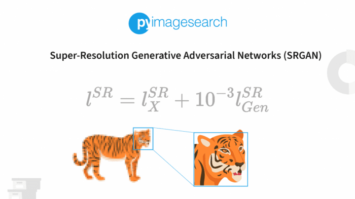
To understand the importance of super-resolution, one look around today’s technology world will automatically explain it. From preserving old media material (films and series) to enhancing a microscope’s view, super-resolution’s impact is widespread and extremely evident. A robust super-resolution algorithm is extremely important in today’s world.

Since the introduction of generative adversarial networks (GANs) took the deep learning world by storm, it was only a matter of time before a super-resolution technique combined with GAN was introduced.

Today we will learn about SRGAN, an ingenious super-resolution technique that combines the concept of GANs with traditional SR methods.

In this tutorial, you will learn how to implement the SRGAN.

This lesson is the 1st in a 4-part series of GANs 201.

1. Super-Resolution Generative Adversarial Networks (SRGAN) (this tutorial)
2. Enhanced Super-Resolution Generative Adversarial Networks (ESRGAN)
3. Pix2Pix GAN for Image-to-Image Translation
4. CycleGAN for Image-to-Image Translation

To learn how to implement SRGANs, just keep reading.

---

Super-Resolution Generative Adversarial Networks (SRGAN)

Although the GANs are in itself a revolutionary concept, their field of application is still fairly new territory. Introducing GANs in super-resolution wasn’t as simple as it sounds. Simply adding the mathematics behind GANs in a super-resolution-like architecture will not accomplish our goal.

The idea of SRGAN was conceived by combining the elements of efficient sub-pixel nets, as well as traditional GAN loss functions. Before we dive deeper into this, Let’s first go through a brief recap of generative adversarial networks.

---

A Brief Recap of GANs

The idea of GAN is best described with the most common example of the detective and the counterfeiter (Figure 1).

The counterfeiter tries to produce realistic art pieces, while the detective distinguishes fake art from real ones. The counterfeiter is the generator, and the detective is the discriminator.

An ideal training will generate data that will fool the discriminator into believing that the data belongs to the training dataset.

Note: The most important intuition about GANs is that the data produced by the generator doesn’t have to be a replica of the training data, but it has to look like it belongs to the training data distribution.

---

Super-Resolution Using GANs

The core concept of GANs is retained in SRGANs (i.e., the min-max function), which makes the generator and discriminator learn in unison by working against each other. SRGAN brings in a few of its own exclusive additions, built on previous research done in this field. Let’s first view the complete architecture of the SRGAN (Figure 2).

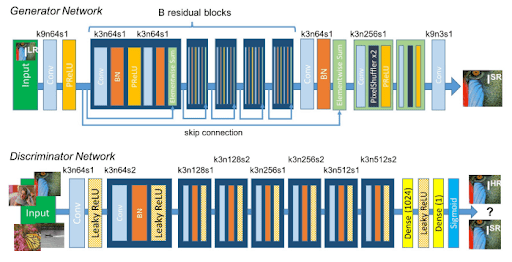
Some key points to note:

• The generator network employs residual blocks, where the idea is to keep information from previous layers alive and allow the network to choose from more features adaptively.
• Instead of adding random noise as the generator input, we pass the low-resolution image.

The discriminator network is pretty standard and works as a discriminator would work in a normal GAN.

The standout factor in SRGANs is the perceptual loss function. While the generator and discriminator will get trained based on the GAN architecture, SRGANs use the help of another loss function to reach their destination: the perceptual/content loss function.

The idea is that SRGAN designs a loss function that reaches its goal by also figuring out the perceptually relevant characteristics. So not only is the adversarial loss helping adjust the weights, but the content loss is also doing its part.

The content loss is defined as VGG loss, which means then a pretrained VGG network output is compared pixel-wise. The only way that the real image VGG output and the fake image VGG output will be similar is when the input images themselves are similar. The intuition behind this is that pixel-wise comparison will help compound the core objective of achieving super-resolution.

When the GAN loss and the content loss are combined, the results are really positive. Our generated super-resolution images are extremely sharp and reflective of their high-resolution (hr) counterparts.

In our project, to show the prowess of the SRGAN, we will be comparing it to a pretrained generator and the original high-resolution image. To make our training more efficient, we will be converting our data into TFRecords.

---

Configuring Your Development Environment

To follow this guide, you need to have the OpenCV library installed on your system.

Luckily, OpenCV is pip-installable:

$ pip install opencv-contrib-python
$ pip install tensorflow

If you need help configuring your development environment for OpenCV, we highly recommend that you read our pip install OpenCV guide — it will have you up and running in a matter of minutes.

---

Having Problems Configuring Your Development Environment?

All that said, are you:

• Short on time?
• Learning on your employer’s administratively locked system?
• Wanting to skip the hassle of fighting with the command line, package managers, and virtual environments?
• Ready to run the code right now on your Windows, macOS, or Linux system?

Then join PyImageSearch University today!

Gain access to Jupyter Notebooks for this tutorial and other PyImageSearch guides that are pre-configured to run on Google Colab’s ecosystem right in your web browser! No installation required.

And best of all, these Jupyter Notebooks will run on Windows, macOS, and Linux!

---

Project Structure

We first need to review our project directory structure.

Start by accessing the “Downloads” section of this tutorial to retrieve the source code and example images.

From there, take a look at the directory structure:

!tree .
.
├── create_tfrecords.py
├── inference.py
├── outputs
├── pyimagesearch
│   ├── config.py
│   ├── data_preprocess.py
│   ├── __init__.py
│   ├── losses.py
│   ├── srgan.py
│   ├── srgan_training.py
│   ├── utils.py
│   └── vgg.py
└── train_srgan.py

2 directories, 11 files

In the pyimagesearch directory, we have:

• config.py: Contains an end-to-end configuration pipeline for the complete project,
• data_preprocess.py: Contains functions to aid in data processing.
• __init__.py: Makes the directory act like a python package.
• losses.py: Initializes the losses required to train the SRGAN.
• srgan.py: Contains the SRGAN architecture.
• srgan_training.py: Contains the training class which runs the SRGAN training.
• utils.py: Contains additional utility
• vgg.py: Initializes a VGG model for perception loss calculation.

In the root directory, we have:

• create_tfrecords.py: Creates TFRecords from the dataset we will use.
• inference.py: Draws inference using the trained models.
• train_srgan.py: Executes the SRGAN training using the srgan.py and srgan_training.py scripts.

---

Creating the Configuration Pipeline

There are a lot of factors that are coming into play while implementing SRGAN. For that, we have created a global configuration file to be used throughout the project. Let’s move to the config.py file located in the pyimagesearch directory.

# import the necessary packages
import os

# name of the TFDS dataset we will be using
DATASET = "div2k/bicubic_x4"

# define the shard size and batch size
SHARD_SIZE = 256
TRAIN_BATCH_SIZE = 64
INFER_BATCH_SIZE = 8

# dataset specs
HR_SHAPE = [96, 96, 3]
LR_SHAPE = [24, 24, 3]
SCALING_FACTOR = 4

# GAN model specs
FEATURE_MAPS = 64
RESIDUAL_BLOCKS = 16
LEAKY_ALPHA = 0.2
DISC_BLOCKS = 4

# training specs
PRETRAIN_LR = 1e-4
FINETUNE_LR = 1e-5
PRETRAIN_EPOCHS = 2500
FINETUNE_EPOCHS = 2500
STEPS_PER_EPOCH = 10

On Line 5, the TFDS dataset is referenced. We are going to use the div2k dataset for our project. The purpose of this dataset is to aid in image super-resolution research, as it contains a variety of high-resolution images.

On Line 8, we have defined the shard size, which is required to create TFRecords. This is followed by the training and inference batch sizes on Lines 9 and 10.

On Line 13, the high-resolution image shape is defined. This is our output shape to which the image will be upscaled. The next variable defined is the low-resolution shape, which will act as our input (Line 14).

Accordingly, the scaling factor is defined as 4 (96/24) (Line 15).

On Lines 18-21, the GAN model specs are defined. These are:

• FEATURE_MAPS: Define the filter size for the CNNs
• RESIDUAL_BLOCKS: As explained earlier, the generator utilizes residual blocks, which defines the number of residual blocks
• LEAKY_ALPHA: Define the alpha parameter for our activation function value
• DISC_BLOCKS: Define the blocks for the discriminator

Then we define the training parameters (Lines 24-28), which include:

• PRETRAIN_LR: The learning rate defines pretraining.
• FINETUNE_LR: The learning rate to be used for fine-tuning
• PRETRAIN_EPOCHS: The number of epochs defined as pretraining
• FINETUNE_EPOCHS: The number of epochs to be used for fine-tuning
• STEPS_PER_EPOCH: Define the number of steps to run per epoch

# define the path to the dataset
BASE_DATA_PATH = "dataset"
DIV2K_PATH = os.path.join(BASE_DATA_PATH, "div2k")

# define the path to the tfrecords for GPU training
GPU_BASE_TFR_PATH = "tfrecord"
GPU_DIV2K_TFR_TRAIN_PATH = os.path.join(GPU_BASE_TFR_PATH, "train")
GPU_DIV2K_TFR_TEST_PATH = os.path.join(GPU_BASE_TFR_PATH, "test")

# define the path to the tfrecords for TPU training
TPU_BASE_TFR_PATH = "gs://<PATH_TO_GCS_BUCKET>/tfrecord"
TPU_DIV2K_TFR_TRAIN_PATH = os.path.join(TPU_BASE_TFR_PATH, "train")
TPU_DIV2K_TFR_TEST_PATH = os.path.join(TPU_BASE_TFR_PATH, "test")

# path to our base output directory
BASE_OUTPUT_PATH = "outputs"

# GPU training SRGAN model paths
GPU_PRETRAINED_GENERATOR_MODEL = os.path.join(BASE_OUTPUT_PATH,
    "models", "pretrained_generator")
GPU_GENERATOR_MODEL = os.path.join(BASE_OUTPUT_PATH, "models",
    "generator")

# TPU training SRGAN model paths
TPU_OUTPUT_PATH = "gs://<PATH_TO_GCS_BUCKET>/outputs"
TPU_PRETRAINED_GENERATOR_MODEL = os.path.join(TPU_OUTPUT_PATH,
    "models", "pretrained_generator")
TPU_GENERATOR_MODEL = os.path.join(TPU_OUTPUT_PATH, "models",
    "generator")

# define the path to the inferred images and to the grid image
BASE_IMAGE_PATH = os.path.join(BASE_OUTPUT_PATH, "images")
GRID_IMAGE_PATH = os.path.join(BASE_IMAGE_PATH, "grid.png")

On Lines 31 and 32, we have defined the reference path to our stored dataset.

Since we will be training our data both on GPU and TPU, we have separately created tfrecords for each training choice. As you know, this project is data-intensive. Hence, it is required to convert our data to tfrecords for optimized and faster training.

First, we have defined the path to the tfrecords for GPU training data (Lines 35-37). This is followed by the definition of the tfrecords referencing the TPU training data (Lines 40-42).

With our training and inference data paths done, we have defined the global output directory on Line 45.

We will compare a pretrained backbone with our fully trained generator model. We define the GPU pretrained generator and the normal generator on Lines 48-51.

As previously mentioned, since we will also be training on TPU, we define separate TPU trained outputs and generator paths on Lines 54-58.

Finally, we add the inferred image subdirectory as well as the grid image subdirectory on Lines 61 and 62 to end our config.py script.

---

Building the Data Processing Pipeline

Since data is undeniably the most important puzzle piece of our project, we have to build an extensive data processing pipeline to deal with all our requirements which involves several data augmentation methods. For that, let’s move into data_preprocess.py in the pyimagesearch directory.

We have created a series of functions that will help us augment our dataset.

# import the necessary packages
from tensorflow.io import FixedLenFeature
from tensorflow.io import parse_single_example
from tensorflow.io import parse_tensor
from tensorflow.image import flip_left_right
from tensorflow.image import rot90
import tensorflow as tf

# define AUTOTUNE object
AUTO = tf.data.AUTOTUNE

def random_crop(lrImage, hrImage, hrCropSize=96, scale=4):
    # calculate the low resolution image crop size and image shape
    lrCropSize = hrCropSize // scale
    lrImageShape = tf.shape(lrImage)[:2]

    # calculate the low resolution image width and height offsets
    lrW = tf.random.uniform(shape=(),
        maxval=lrImageShape[1] - lrCropSize + 1, dtype=tf.int32)
    lrH = tf.random.uniform(shape=(),
        maxval=lrImageShape[0] - lrCropSize + 1, dtype=tf.int32)

    # calculate the high resolution image width and height
    hrW = lrW * scale
    hrH = lrH * scale

    # crop the low and high resolution images
    lrImageCropped = tf.slice(lrImage, [lrH, lrW, 0], 
        [(lrCropSize), (lrCropSize), 3])
    hrImageCropped = tf.slice(hrImage, [hrH, hrW, 0],
        [(hrCropSize), (hrCropSize), 3])

    # return the cropped low and high resolution images
    return (lrImageCropped, hrImageCropped)

Considering the amount of TensorFlow wrappers we will use in this project, defining a tf.data.AUTOTUNE object for space optimization is a good approach.

The first function we have defined is random_crop (Line 12). It takes in the following arguments:

• lrImage: The low-resolution image.
• hrImage: The high-resolution image.
• hrCropSize: The high-resolution crop size for low-resolution crop calculation.
• scale: The factor by which we calculate the low-resolution crop.

Using tf.random.uniform, we calculate the low-resolution (lr) width and height offsets on Lines 18-21.

To calculate the corresponding high-resolution values, we simply multiply the low-resolution values with the scale factor (Lines 24 and 25).

Using the values, we crop out the low-resolution image and its corresponding high-resolution crop and return them (Lines 28-34).

def get_center_crop(lrImage, hrImage, hrCropSize=96, scale=4):
    # calculate the low resolution image crop size and image shape
    lrCropSize = hrCropSize // scale
    lrImageShape = tf.shape(lrImage)[:2]

    # calculate the low resolution image width and height
    lrW = lrImageShape[1] // 2
    lrH = lrImageShape[0] // 2

    # calculate the high resolution image width and height
    hrW = lrW * scale
    hrH = lrH * scale

    # crop the low and high resolution images
    lrImageCropped = tf.slice(lrImage, [lrH - (lrCropSize // 2),
        lrW - (lrCropSize // 2), 0], [lrCropSize, lrCropSize, 3])
    hrImageCropped = tf.slice(hrImage, [hrH - (hrCropSize // 2),
        hrW - (hrCropSize // 2), 0], [hrCropSize, hrCropSize, 3])

    # return the cropped low and high resolution images
    return (lrImageCropped, hrImageCropped)

Our next function under the spotlight is get_center_crop (Line 36), which takes in the following arguments:

• lrImage: The low-resolution image
• hrImage: The high-resolution image
• hrCropSize: The high-resolution crop size for low-resolution crop calculation
• scale: The factor by which we calculate the low-resolution crop

Just like we created crop size values for our previous function, we get the lr crop size values and image shape on Lines 38 and 39.

On Lines 42 and 43, we divide the low-resolution shape by 2 and get the center points.

To get the corresponding high-resolution center points, multiply the lr center points by the scale factor (Lines 46 and 47).

On Lines 50-53, we get center crops of low-resolution and high-resolution images and return them.

def random_flip(lrImage, hrImage):
    # calculate a random chance for flip
    flipProb = tf.random.uniform(shape=(), maxval=1)
    (lrImage, hrImage) = tf.cond(flipProb < 0.5,
        lambda: (lrImage, hrImage),
        lambda: (flip_left_right(lrImage), flip_left_right(hrImage)))
    
    # return the randomly flipped low and high resolution images
    return (lrImage, hrImage)

On Line 58, we have the random_flip function to flip images. It takes in the low-resolution and high-resolution images as its arguments.

Based on a flip probability value using tf.random.uniform, we flip our images and return them.

def random_rotate(lrImage, hrImage):
    # randomly generate the number of 90 degree rotations
    n = tf.random.uniform(shape=(), maxval=4, dtype=tf.int32)

    # rotate the low and high resolution images
    lrImage = rot90(lrImage, n)
    hrImage = rot90(hrImage, n)

    # return the randomly rotated images
    return (lrImage, hrImage)

The random_rotate function on Line 68 will randomly rotate the pair of high-resolution and low-resolution images based on a value generated by tf.random.uniform (Lines 70-77).

def read_train_example(example):
    # get the feature template and  parse a single image according to
    # the feature template
    feature = {
        "lr": FixedLenFeature([], tf.string),
        "hr": FixedLenFeature([], tf.string),
    }
    example = parse_single_example(example, feature)

    # parse the low and high resolution images
    lrImage = parse_tensor(example["lr"], out_type=tf.uint8)
    hrImage = parse_tensor(example["hr"], out_type=tf.uint8)

The read_train_example function takes in a single example image set (an lr and an hr image collection) as an argument (Line 79). On Lines 82-85, we create a feature template.

We parse the low-resolution and the high-resolution images from the example set (Lines 86-90).

    # perform data augmentation
    (lrImage, hrImage) = random_crop(lrImage, hrImage)
    (lrImage, hrImage) = random_flip(lrImage, hrImage)
    (lrImage, hrImage) = random_rotate(lrImage, hrImage)

    # reshape the low and high resolution images
    lrImage = tf.reshape(lrImage, (24, 24, 3))
    hrImage = tf.reshape(hrImage, (96, 96, 3))

    # return the low and high resolution images
    return (lrImage, hrImage)

Using our previously created function, we apply data augmentation to our example image sets (Lines 93-95).

Once our images are augmented, we reshape the images to our required input and output sizes (Lines 98 and 99).

def read_test_example(example):
    # get the feature template and  parse a single image according to
    # the feature template
    feature = {
        "lr": FixedLenFeature([], tf.string),
        "hr": FixedLenFeature([], tf.string),
    }
    example = parse_single_example(example, feature)

    # parse the low and high resolution images
    lrImage = parse_tensor(example["lr"], out_type=tf.uint8)
    hrImage = parse_tensor(example["hr"], out_type=tf.uint8)

    # center crop both low and high resolution image
    (lrImage, hrImage) = get_center_crop(lrImage, hrImage)

    # reshape the low and high resolution images
    lrImage = tf.reshape(lrImage, (24, 24, 3))
    hrImage = tf.reshape(hrImage, (96, 96, 3))

    # return the low and high resolution images
    return (lrImage, hrImage)

We create a similar function, read_test_example, to read an inference image set. All steps are repeated from the previously created read_train_example. The exception is that since this is for our inference, we do not apply any augmentation to the data (Lines 104-125).

def load_dataset(filenames, batchSize, train=False):
    # get the TFRecords from the filenames
    dataset = tf.data.TFRecordDataset(filenames, 
        num_parallel_reads=AUTO)

    # check if this is the training dataset
    if train:
        # read the training examples
        dataset = dataset.map(read_train_example,
            num_parallel_calls=AUTO)
    # otherwise, we are working with the test dataset
    else:
        # read the test examples
        dataset = dataset.map(read_test_example,
            num_parallel_calls=AUTO)

    # batch and prefetch the data
    dataset = (dataset
        .shuffle(batchSize)
        .batch(batchSize)
        .repeat()
        .prefetch(AUTO)
    )

    # return the dataset
    return dataset

The final function in our data processing pipeline script is load_dataset (Line 127), which takes in the following arguments:

• filenames: Names of the files being considered
• batchSize: To define the batch size to be considered at a time
• train: A bool variable that tells us if the mode is set to training

On Line 129, we use tf.data to get TFRecords from the filenames.

If the mode is set to train, we map the read_train_example function to our dataset (Lines 133-136). This means that all records inside the dataset get passed through the function.

If the mode is set to anything else, we map the read_test_example function to our dataset (Lines 138-141).

Our final step is to batch and prefetch the dataset (Lines 144-149).

---

Implementing the SRGAN Loss Functions

Although our actual loss calculation will be done later, a simple utility script to store loss functions will help organize our project better. Since we do not need to write the mathematical equations for the losses (TensorFlow does that for us), we just need to call the required packages.

For that, let’s move into the losses.py script located in the pyimagesearch directory.

# import necessary packages
from tensorflow.keras.losses import MeanSquaredError
from tensorflow.keras.losses import BinaryCrossentropy
from tensorflow.keras.losses import Reduction
from tensorflow import reduce_mean

class Losses:
    def __init__(self, numReplicas):
        self.numReplicas = numReplicas

    def bce_loss(self, real, pred):
        # compute binary cross entropy loss without reduction
        BCE = BinaryCrossentropy(reduction=Reduction.NONE)
        loss = BCE(real, pred)

        # compute reduced mean over the entire batch
        loss = reduce_mean(loss) * (1. / self.numReplicas)

        # return reduced bce loss
        return loss

A complete class dedicated to losses is created (Line 7). We first define the binary cross entropy loss function on Line 11, which takes in the real and predicted values.

A binary cross entropy object is created, and the loss is calculated (Lines 13 and 14). The loss is then calculated over the entire batch (Line 17).

    def mse_loss(self, real, pred):
        # compute mean squared error loss without reduction
        MSE = MeanSquaredError(reduction=Reduction.NONE)
        loss = MSE(real, pred)

        # compute reduced mean over the entire batch
        loss = reduce_mean(loss) * (1. / self.numReplicas)

        # return reduced mse loss
        return loss

Next, a mean squared error loss function on Line 22 is defined. An MSE object is created, and the loss is calculated (Lines 24 and 25).

As done in the previous function, we calculate the loss over the entire batch and return it (Lines 28-31).

---

Implementing the SRGAN

To start implementing the SRGAN architecture, let us move to srgan.py located in the pyimagesearch directory.

# import the necessary packages
from tensorflow.keras.layers import BatchNormalization
from tensorflow.keras.layers import GlobalAvgPool2D
from tensorflow.keras.layers import LeakyReLU
from tensorflow.keras.layers import Rescaling
from tensorflow.keras.layers import Conv2D
from tensorflow.keras.layers import Dense
from tensorflow.keras.layers import PReLU
from tensorflow.keras.layers import Add
from tensorflow.nn import depth_to_space
from tensorflow.keras import Model
from tensorflow.keras import Input

class SRGAN(object):
    @staticmethod
    def generator(scalingFactor, featureMaps, residualBlocks):
        # initialize the input layer
        inputs = Input((None, None, 3))
        xIn = Rescaling(scale=(1.0 / 255.0), offset=0.0)(inputs)

To encompass our generator and discriminator, we create a class called SRGAN (Line 14).

First, we define our generator function on Line 16, which takes in the following arguments:

• scalingFactor: Required to get our final upscaled output.
• featureMaps: Determines the number of convolution filters we want.
• residualBlocks: Determines the number of residual connection blocks we want.

On Lines 18 and 19, we define the input to our generator and rescale the pixels to the range of 0 and 1.

        # pass the input through CONV => PReLU block
        xIn = Conv2D(featureMaps, 9, padding="same")(xIn)
        xIn = PReLU(shared_axes=[1, 2])(xIn)

        # construct the "residual in residual" block
        x = Conv2D(featureMaps, 3, padding="same")(xIn)
        x = BatchNormalization()(x)
        x = PReLU(shared_axes=[1, 2])(x)
        x = Conv2D(featureMaps, 3, padding="same")(x)
        x = BatchNormalization()(x)
        xSkip = Add()([xIn, x])

We first pass the input through the Conv2D layer and a parametric ReLU layer (Lines 22 and 23).

Next, we build a base residual block network. A Conv2D layer, a batch normalization layer, followed by a parametric ReLU layer, a Conv2D layer, and another batch normalization layer (Lines 26-30).

The final step here is to add our input xIn with the residual block output x to finish the residual block network (Line 31).

        # create a number of residual blocks
        for _ in range(residualBlocks - 1):
            x = Conv2D(featureMaps, 3, padding="same")(xSkip)
            x = BatchNormalization()(x)
            x = PReLU(shared_axes=[1, 2])(x)
            x = Conv2D(featureMaps, 3, padding="same")(x)
            x = BatchNormalization()(x)
            xSkip = Add()([xSkip, x])
        
        # get the last residual block without activation
        x = Conv2D(featureMaps, 3, padding="same")(xSkip)
        x = BatchNormalization()(x)
        x = Add()([xIn, x])

We automate the residual block entries using a for loop and essentially repeat the process of the base residual block (Lines 34-40).

Once outside the loop, we add the final Conv2D and batch normalization layer before adding the skip connection (Lines 43-45).

        # upscale the image with pixel shuffle
        x = Conv2D(featureMaps * (scalingFactor // 2), 3, padding="same")(x)
        x = depth_to_space(x, 2)
        x = PReLU(shared_axes=[1, 2])(x)

        # upscale the image with pixel shuffle
        x = Conv2D(featureMaps * scalingFactor, 3,
            padding="same")(x)
        x = depth_to_space(x, 2)
        x = PReLU(shared_axes=[1, 2])(x)

        # get the output and scale it from [-1, 1] to [0, 255] range
        x = Conv2D(3, 9, padding="same", activation="tanh")(x)
        x = Rescaling(scale=127.5, offset=127.5)(x)
    
        # create the generator model
        generator = Model(inputs, x)

        # return the generator
        return generator

Our inputs are passed through a Conv2D layer where the scaling factor value comes into play (Line 48).

The depth_to_space function is a beautiful utility function provided by TensorFlow, which rearranges the pixels of our input, expanding them height- and width-wise by decreasing the channel value (Line 49).

This is followed by a parametric ReLU function, which is followed by a repeat of the Conv2D, depth_to_space, and another parametric ReLU function (Lines 50-56).

Notice that the Conv2D function on Line 59 has tanh as its activation function. That means that the feature maps’ values are now scaled to the range of -1 and 1. We rescale the values using Rescaling (Line 60) and get the pixels back to the range of 0 to 255.

That concludes our generator, so we simply initialize the generator and return it (Lines 63-66).

    @staticmethod
    def discriminator(featureMaps, leakyAlpha, discBlocks):
        # initialize the input layer and process it with conv kernel
        inputs = Input((None, None, 3))
        x = Rescaling(scale=(1.0 / 127.5), offset=-1.0)(inputs)
        x = Conv2D(featureMaps, 3, padding="same")(x)
        
        # unlike the generator we use leaky relu in the discriminator
        x = LeakyReLU(leakyAlpha)(x)

        # pass the output from previous layer through a CONV => BN =>
        # LeakyReLU block
        x = Conv2D(featureMaps, 3, padding="same")(x)
        x = BatchNormalization()(x)
        x = LeakyReLU(leakyAlpha)(x)

We move on to the discriminator, for which we have defined a function on Line 69. It takes in the following arguments:

• featureMaps: Determines the number of filters inside a Conv2D layer.
• leakyAlpha: The value to be provided into the leaky ReLU activation function,
• discBlocks: Number of discriminator blocks to be added inside the architecture.

The inputs to the discriminator are first defined. Then they are followed by rescaling the pixels to the range of -1 to 1 (Lines 71 and 72). This is followed by a Conv2D layer and a LeakyReLU activation layer on Lines 73-76.

Next, we create a combination of 3 layers: the Conv2D layer followed by batch normalization, ending with a LeakyReLU function (Lines 80-82). You’ll see that this combination is repeated a lot.

        # create a number of discriminator blocks
        for i in range(1, discBlocks):
            # first CONV => BN => LeakyReLU block
            x = Conv2D(featureMaps * (2 ** i), 3, strides=2,
                padding="same")(x)
            x = BatchNormalization()(x)
            x = LeakyReLU(leakyAlpha)(x)

            # second CONV => BN => LeakyReLU block
            x = Conv2D(featureMaps * (2 ** i), 3, padding="same")(x)
            x = BatchNormalization()(x)
            x = LeakyReLU(leakyAlpha)(x)

Based on the previous discBlocks value, we start a loop and keep adding discriminator blocks. Each discriminator block contains the Conv2D → BatchNormalization → LeakyReLU combination repeated twice (Lines 85-95).

        # process the feature maps with global average pooling
        x = GlobalAvgPool2D()(x)
        x = LeakyReLU(leakyAlpha)(x)

        # final FC layer with sigmoid activation function
        x = Dense(1, activation="sigmoid")(x)

        # create the discriminator model
        discriminator = Model(inputs, x)

        # return the discriminator
        return discriminator

Outside the loop, we add a global average pooling layer, followed by another LeakyReLU activation function (Lines 98 and 99).

Since the discriminator gives us the information about the authenticity of an input, the final layer of our network is a Dense layer with a sigmoid activation function (Lines 102).

---

Implementing the SRGAN Training Script

As explained at the beginning of this blog, the SRGAN training requires two losses at the same time; the VGG content loss as well as the GAN loss. Let’s move into the srgan_training script inside the pyimagesearch directory.

# import the necessary packages
from tensorflow.keras import Model
from tensorflow import GradientTape
from tensorflow import concat
from tensorflow import zeros
from tensorflow import ones
import tensorflow as tf

class SRGANTraining(Model):
    def __init__(self, generator, discriminator, vgg, batchSize):
        super().__init__()
        # initialize the generator, discriminator, vgg model, and 
        # the global batch size
        self.generator = generator
        self.discriminator = discriminator
        self.vgg = vgg
        self.batchSize = batchSize

To make our lives easier, we have gone ahead and created a class for the SRGAN training on Line 9.

The __init__ function of this class takes in the following arguments (Line 10):

• generator: The generator of the SRGAN
• discriminator: The discriminator of the SRGAN
• vgg: The VGG network to be used for the content loss
• batchSize: The batch size to be used during training

On Lines 14-17, we simply initialize the generator, discriminator, VGG, and batch size values of the class by assigning them to the arguments.

    def compile(self, gOptimizer, dOptimizer, bceLoss, mseLoss):
        super().compile()
        # initialize the optimizers for the generator 
        # and discriminator
        self.gOptimizer = gOptimizer
        self.dOptimizer = dOptimizer
        
        # initialize the loss functions
        self.bceLoss = bceLoss
        self.mseLoss = mseLoss

On Line 19, we define the compile function of our SRGAN. It takes in the following arguments:

• gOptimizer: Optimizer for the generator
• dOptimzer: Optimizer for the discriminator
• bceLoss: The binary cross entropy loss
• mseLoss: The mean squared error loss

The rest of the function initializes the corresponding class variables (Lines 23-28).

    def train_step(self, images):
        # grab the low and high resolution images
        (lrImages, hrImages) = images
        lrImages = tf.cast(lrImages, tf.float32)
        hrImages = tf.cast(hrImages, tf.float32)

        # generate super resolution images
        srImages = self.generator(lrImages)

        # combine them with real images
        combinedImages = concat([srImages, hrImages], axis=0)

        # assemble labels discriminating real from fake images where
        # label 0 is for predicted images and 1 is for original high
        # resolution images
        labels = concat(
            [zeros((self.batchSize, 1)), ones((self.batchSize, 1))],
            axis=0)

On Line 30, we define the train_step, which takes in the training images as its argument.

We proceed to unpack the images and turn them into float type (Lines 32-34).

Passing the low-resolution images through the generator, we obtain our fake super-resolution images. These are combined with the true super-resolution images on Line 40.

For our discriminator training, we have to create labels for this combined set of images. The fake images generated by the generator will have a label of 0, while the real high-resolution images will have a label of 1 (Lines 45-47).

        # train the discriminator
        with GradientTape() as tape:
            # get the discriminator predictions
            predictions = self.discriminator(combinedImages)
            
            # compute the loss
            dLoss = self.bceLoss(labels, predictions)
        
        # compute the gradients
        grads = tape.gradient(dLoss,
            self.discriminator.trainable_variables)
        
        # optimize the discriminator weights according to the
        # gradients computed
        self.dOptimizer.apply_gradients(
            zip(grads, self.discriminator.trainable_variables)
        )

        # generate misleading labels
        misleadingLabels = ones((self.batchSize, 1))

To train the discriminator, the GradientTape is turned on for backpropagation (Line 50).

The combined image set is passed through the discriminator for predictions (Line 52). Using the bceLoss, we calculate the discriminator loss by comparing them to the labels (Line 55).

We compute the gradients and optimize the weights according to the gradients (Lines 58-65).

For the generator weight calculations, we have to label the images generated by the generator as real (Line 68).

        # train the generator (note that we should *not* update the
        #  weights of the discriminator)!
        with GradientTape() as tape:
            # get fake images from the generator
            fakeImages = self.generator(lrImages)
        
            # get the prediction from the discriminator
            predictions = self.discriminator(fakeImages)
        
            # compute the adversarial loss
            gLoss = 1e-3 * self.bceLoss(misleadingLabels, predictions)
            
            # compute the normalized vgg outputs
            srVgg = tf.keras.applications.vgg19.preprocess_input(
                fakeImages)
            srVgg = self.vgg(srVgg) / 12.75
            hrVgg = tf.keras.applications.vgg19.preprocess_input(
                hrImages)
            hrVgg = self.vgg(hrVgg) / 12.75

            # compute the perceptual loss
            percLoss = self.mseLoss(hrVgg, srVgg)
        
            # calculate the total generator loss
            gTotalLoss = gLoss + percLoss
        
        # compute the gradients
        grads = tape.gradient(gTotalLoss,
            self.generator.trainable_variables)
        
        # optimize the generator weights with the computed gradients
        self.gOptimizer.apply_gradients(zip(grads,
            self.generator.trainable_variables)
        )

        # return the generator and discriminator losses
        return {"dLoss": dLoss, "gTotalLoss": gTotalLoss,
            "gLoss": gLoss, "percLoss": percLoss}

On Line 72, we start another GradientTape for the generator.

On Line 74, we generate the fake high-resolution images from the low-resolution images passed through the generator.

These fake images are passed through the discriminator to get our predictions. These predictions are compared against the misleading labels to get our binary cross entropy loss on Line 80.

For the content loss, we pass the fake super-resolution images and the actual high-resolution images through a VGG net and compare them using our mean squared loss function (Lines 83-91).

As explained earlier, the total generator loss becomes the sum of the generative loss and the content loss (Line 94).

Next, we calculate the gradients for the generator and apply them (Lines 97-103).

This concludes our SRGAN training module.

---

Implementing the Final Utility Scripts

As you can figure out from the srgan_training script, we have used a few helper scripts. Let’s quickly go over them before assessing our outputs.

First, let’s move to the vgg.py script located in the pyimagesearch directory.

# import the necessary packages
from tensorflow.keras.applications import VGG19
from tensorflow.keras import Model

class VGG:
    @staticmethod
    def build():
        # initialize the pre-trained VGG19 model
        vgg = VGG19(input_shape=(None, None, 3), weights="imagenet",
            include_top=False)

        # slicing the VGG19 model till layer #20
        model = Model(vgg.input, vgg.layers[20].output)

        # return the sliced VGG19 model
        return model

Inside it, we define a class called VGG on Line 5. The build function defined on Line 7 uses tensorflow packages to call a pretrained VGG model and use it for our content loss (Lines 9-16).

We just have another script to check before finalizing the training. To aid in assessing our output images, we have created a zoom-in script. For that, let’s move into the utils.py located in the pyimagesearch directory.

# import the necessary packages
from . import config
from matplotlib.pyplot import subplots
from matplotlib.pyplot import savefig
from matplotlib.pyplot import title
from matplotlib.pyplot import xticks
from matplotlib.pyplot import yticks
from matplotlib.pyplot import show
from tensorflow.keras.preprocessing.image import array_to_img
from mpl_toolkits.axes_grid1.inset_locator import zoomed_inset_axes
from mpl_toolkits.axes_grid1.inset_locator import mark_inset
import os

# the following code snippet has been taken from:
# https://keras.io/examples/vision/super_resolution_sub_pixel
def zoom_into_images(image, imageTitle):
    # create a new figure with a default 111 subplot.
    (fig, ax) = subplots()
    im = ax.imshow(array_to_img(image[::-1]), origin="lower")

    title(imageTitle)
    # zoom-factor: 2.0, location: upper-left
    axins = zoomed_inset_axes(ax, 2, loc=2)
    axins.imshow(array_to_img(image[::-1]), origin="lower")

    # specify the limits.
    (x1, x2, y1, y2) = 20, 40, 20, 40
    # apply the x-limits.
    axins.set_xlim(x1, x2)
    # apply the y-limits.
    axins.set_ylim(y1, y2)

    # remove the xticks and yticks
    yticks(visible=False)
    xticks(visible=False)

    # make the line.
    mark_inset(ax, axins, loc1=1, loc2=3, fc="none", ec="blue")

    # build the image path and save it to disk
    imagePath = os.path.join(config.BASE_IMAGE_PATH,
        f"{imageTitle}.png")
    savefig(imagePath)
    
    # show the image
    show()

We implement our zoom_into_images function on Line 16. It takes in the image and image title as its arguments.

A subplot for multiple plots is defined on Line 18. The image is plotted on Line 19. On Lines 21-24, we plot the same image but with a particular patch zoomed in for our reference.

On Lines 26-31, we specify the x and y coordinates limits for the image.

The rest of the function involves some decorations, like removing the ticks, adding the lines, and saving the image to our output path (Lines 34-46).

---

Training the SRGAN

With all our required scripts complete, the final step is to execute the training process. For that, let’s head into the train_srgan.py script inside our root directory.

# USAGE
# python train_srgan.py --device tpu
# python train_srgan.py --device gpu

# import tensorflow and fix the random seed for better reproducibility
import tensorflow as tf
tf.random.set_seed(42)

# import the necessary packages
from pyimagesearch.data_preprocess import load_dataset
from pyimagesearch.srgan import SRGAN
from pyimagesearch.vgg import VGG
from pyimagesearch.srgan_training import SRGANTraining
from pyimagesearch import config
from pyimagesearch.losses import Losses
from tensorflow import distribute
from tensorflow.config import experimental_connect_to_cluster
from tensorflow.tpu.experimental import initialize_tpu_system
from tensorflow.keras.optimizers import Adam
from tensorflow.io.gfile import glob
import argparse
import sys
import os

# construct the argument parser and parse the arguments
ap = argparse.ArgumentParser()
ap.add_argument("--device", required=True, default="gpu",
    choices=["gpu", "tpu"], type=str,
    help="device to use for training (gpu or tpu)")
args = vars(ap.parse_args())

An argument parser is created to take in the device choice input from the user (Lines 26-30).

# check if we are using TPU, if so, initialize the TPU strategy
if args["device"] == "tpu":
    # initialize the TPUs
    tpu = distribute.cluster_resolver.TPUClusterResolver() 
    experimental_connect_to_cluster(tpu)
    initialize_tpu_system(tpu)
    strategy = distribute.TPUStrategy(tpu)

    # ensure the user has entered a valid gcs bucket path
    if config.TPU_BASE_TFR_PATH == "gs://<PATH_TO_GCS_BUCKET>/tfrecord":
        print("[INFO] not a valid GCS Bucket path...")
        sys.exit(0)
    
    # set the train TFRecords, pretrained generator, and final
    # generator model paths to be used for TPU training
    tfrTrainPath = config.TPU_DIV2K_TFR_TRAIN_PATH
    pretrainedGenPath = config.TPU_PRETRAINED_GENERATOR_MODEL
    genPath = config.TPU_GENERATOR_MODEL

# otherwise, we are using multi/single GPU so initialize the mirrored
# strategy
elif args["device"] == "gpu":
    # define the multi-gpu strategy
    strategy = distribute.MirroredStrategy()

    # set the train TFRecords, pretrained generator, and final
    # generator model paths to be used for GPU training
    tfrTrainPath = config.GPU_DIV2K_TFR_TRAIN_PATH
    pretrainedGenPath = config.GPU_PRETRAINED_GENERATOR_MODEL
    genPath = config.GPU_GENERATOR_MODEL

# else, invalid argument was provided as input
else:
    # exit the program
    print("[INFO] please enter a valid device argument...")
    sys.exit(0)

Since we can train the SRGAN with either the TPU or the GPU, we make arrangements accordingly.

Our first case is if the device is set to tpu, we initialize the requirements for the TPU training (Lines 33-43) :

• TPUClusterResolver: For efficient communication with cluster management systems (AWS, GCP, etc.)
• strategy: To initialize the right strategy for efficient TPU training.

Next, we set the training TFRecords path, pretrained generator path, and the final generator path (Lines 47-49).

If the device is set to gpu, we set the training strategy to be mirrored over multiple GPUs (Lines 53-55).

The GPU TFRecords path, the pretrained generator, and the final generator paths are defined (Lines 59-61). Notice how in each case, these variables are exclusive to the case itself (i.e., GPU_GENERATOR_MODEL or TPU_GENERATOR_MODEL).

If the user gives neither the gpu nor tpu choice, the program simply exits (Lines 64-67).

# display the number of accelerators
print("[INFO] number of accelerators: {}..."
    .format(strategy.num_replicas_in_sync))

# grab train TFRecord filenames
print("[INFO] grabbing the train TFRecords...")
trainTfr = glob(tfrTrainPath +"/*.tfrec")

# build the div2k datasets from the TFRecords
print("[INFO] creating train and test dataset...")
trainDs = load_dataset(filenames=trainTfr, train=True,
    batchSize=config.TRAIN_BATCH_SIZE * strategy.num_replicas_in_sync)

# call the strategy scope context manager
with strategy.scope():
    # initialize our losses class object
    losses = Losses(numReplicas=strategy.num_replicas_in_sync)

    # initialize the generator, and compile it with Adam optimizer and
    # MSE loss
    generator = SRGAN.generator(
        scalingFactor=config.SCALING_FACTOR,
        featureMaps=config.FEATURE_MAPS,
        residualBlocks=config.RESIDUAL_BLOCKS)
    generator.compile(
        optimizer=Adam(learning_rate=config.PRETRAIN_LR),
        loss=losses.mse_loss)

    # pretraining the generator
    print("[INFO] pretraining SRGAN generator...")
    generator.fit(trainDs, epochs=config.PRETRAIN_EPOCHS,
        steps_per_epoch=config.STEPS_PER_EPOCH)

On Lines 70-80, we build the div2k dataset from the TFRecords. Calling the strategy scope, we initialize the loss function from our loss object (Lines 83-85).

The generator is then initialized using values from our config.py script and compiled with the Adam optimizer (Lines 89-95).

For better results, we have pretrained the generator network on Lines 99 and 100.

# check whether output model directory exists, if it doesn't, then
# create it
if args["device"] == "gpu" and not os.path.exists(config.BASE_OUTPUT_PATH):
    os.makedirs(config.BASE_OUTPUT_PATH)

# save the pretrained generator
print("[INFO] saving the SRGAN pretrained generator to {}..."
    .format(pretrainedGenPath))
generator.save(pretrainedGenPath)

# call the strategy scope context manager
with strategy.scope():
    # initialize our losses class object
    losses = Losses(numReplicas=strategy.num_replicas_in_sync)

    # initialize the vgg network (for perceptual loss) and discriminator
    # network
    vgg = VGG.build()
    discriminator = SRGAN.discriminator(
        featureMaps=config.FEATURE_MAPS, 
        leakyAlpha=config.LEAKY_ALPHA, discBlocks=config.DISC_BLOCKS)

    # build the SRGAN training model and compile it
    srgan = SRGANTraining(
        generator=generator,
        discriminator=discriminator,
        vgg=vgg,
        batchSize=config.TRAIN_BATCH_SIZE)
    srgan.compile(
        dOptimizer=Adam(learning_rate=config.FINETUNE_LR),
        gOptimizer=Adam(learning_rate=config.FINETUNE_LR),
        bceLoss=losses.bce_loss,
        mseLoss=losses.mse_loss,
    )

    # train the SRGAN model
    print("[INFO] training SRGAN...")
    srgan.fit(trainDs, epochs=config.FINETUNE_EPOCHS,
        steps_per_epoch=config.STEPS_PER_EPOCH)

# save the SRGAN generator
print("[INFO] saving SRGAN generator to {}...".format(genPath))
srgan.generator.save(genPath)

On Lines 104 and 105, we check if the output path for our outputs exists. If not, we create one.

Once the pretrained generator is saved, we recall the strategy scope and initialize the loss object again (Lines 110-115).

Since we will need the VGG network for our content loss, we initialize a VGG network and the discriminator, the latter with values in the config.py script (Lines 119-122).

Since the generator and discriminator are already created, we have directly used the SRGANTraining object and compiled our SRGAN model (Lines 125-135).

The initialized SRGAN is fit with the data to initiate the training, and the trained SRGAN is then saved (Lines 139-144)

---

Creating the Inference Script for the SRGAN

With our training done, let’s see some results! For that, we’ll be moving to the inference.py script.

# USAGE
# python inference.py --device gpu
# python inference.py --device tpu

# import the necessary packages
from pyimagesearch.data_preprocess import load_dataset
from pyimagesearch.utils import zoom_into_images
from pyimagesearch import config
from tensorflow import distribute
from tensorflow.config import experimental_connect_to_cluster
from tensorflow.tpu.experimental import initialize_tpu_system
from tensorflow.keras.models import load_model
from tensorflow.keras.preprocessing.image import array_to_img
from tensorflow.io.gfile import glob
from matplotlib.pyplot import subplots
import argparse
import sys
import os

# construct the argument parser and parse the arguments
ap = argparse.ArgumentParser()
ap.add_argument("--device", required=True, default="gpu",
    choices=["gpu", "tpu"], type=str,
    help="device to use for training (gpu or tpu)")
args = vars(ap.parse_args())

As done in the training script, we need to create another argument parser that takes the choice of the device (TPU or GPU) from the user (Lines 21-25).

# check if we are using TPU, if so, initialize the strategy
# accordingly
if args["device"] == "tpu":
    # initialize the tpus
    tpu = distribute.cluster_resolver.TPUClusterResolver()
    experimental_connect_to_cluster(tpu)
    initialize_tpu_system(tpu)
    strategy = distribute.TPUStrategy(tpu)

    # ensure the user has entered a valid gcs bucket path
    if config.TPU_BASE_TFR_PATH == "gs://<PATH_TO_GCS_BUCKET>/tfrecord":
        print("[INFO] not a valid GCS Bucket path...")
        sys.exit(0)

    # set the train TFRecords, pretrained generator, and final
    # generator model paths to be used for TPU training
    tfrTestPath = config.TPU_DIV2K_TFR_TEST_PATH
    pretrainedGenPath = config.TPU_PRETRAINED_GENERATOR_MODEL
    genPath = config.TPU_GENERATOR_MODEL

# otherwise, we are using multi/single GPU so initialize the mirrored
# strategy
elif args["device"] == "gpu":
    # define the multi-gpu strategy
    strategy = distribute.MirroredStrategy()

    # set the train TFRecords, pretrained generator, and final
    # generator model paths to be used for GPU training
    tfrTestPath = config.GPU_DIV2K_TFR_TEST_PATH
    pretrainedGenPath = config.GPU_PRETRAINED_GENERATOR_MODEL
    genPath = config.GPU_GENERATOR_MODEL

# else, invalid argument was provided as input
else:
    # exit the program
    print("[INFO] please enter a valid device argument...")
    sys.exit(0)

The next step is again the same as the training step. Depending on the choice of device, we initialize clusters (for TPU), strategies (for both GPU and TPU), and the paths while setting up an exit clause for the script (Lines 27-63).

# get the dataset
print("[INFO] loading the test dataset...")
testTfr = glob(tfrTestPath + "/*.tfrec")
testDs = load_dataset(testTfr, config.INFER_BATCH_SIZE, train=False)

# get the first batch of testing images
(lrImage, hrImage) = next(iter(testDs))

# call the strategy scope context manager
with strategy.scope(): 
    # load the SRGAN trained models
    print("[INFO] loading the pre-trained and fully trained SRGAN model...")
    srganPreGen = load_model(pretrainedGenPath, compile=False)
    srganGen = load_model(genPath, compile=False)
    
    # predict using SRGAN
    print("[INFO] making predictions with pre-trained and fully trained SRGAN model...")
    srganPreGenPred = srganPreGen.predict(lrImage)
    srganGenPred = srganGen.predict(lrImage)

On Lines 67 and 68, we obtain the dataset we use for inference.

Using next(iter()), we get the first batch of testing images (Line 71). Next, the pretrained SRGAN and the fully trained SRGAN model weights are loaded and initialized, with the first low-resolution image being passed through them (Lines 74-83).

# plot the respective predictions
print("[INFO] plotting the SRGAN predictions...")
(fig, axes) = subplots(nrows=config.INFER_BATCH_SIZE, ncols=4,
    figsize=(50, 50))

# plot the predicted images from low res to high res
for (ax, lowRes, srPreIm, srGanIm, highRes) in zip(axes, lrImage,
        srganPreGenPred, srganGenPred, hrImage):
    # plot the low resolution image
    ax[0].imshow(array_to_img(lowRes))
    ax[0].set_title("Low Resolution Image")

    # plot the pretrained SRGAN image
    ax[1].imshow(array_to_img(srPreIm))
    ax[1].set_title("SRGAN Pretrained")

    # plot the SRGAN image
    ax[2].imshow(array_to_img(srGanIm))
    ax[2].set_title("SRGAN")

    # plot the high resolution image
    ax[3].imshow(array_to_img(highRes))
    ax[3].set_title("High Resolution Image")

On Lines 87 and 88, we initialize the subplot. Then, looping over the columns of the subplot, we plot the low-resolution image, the SRGAN pretrained result, the fully SRGAN super-resolution image, and the original high-resolution image (Lines 91-107).

# check whether output image directory exists, if it doesn't, then
# create it
if not os.path.exists(config.BASE_IMAGE_PATH):
    os.makedirs(config.BASE_IMAGE_PATH)

# serialize the results to disk
print("[INFO] saving the SRGAN predictions to disk...")
fig.savefig(config.GRID_IMAGE_PATH)

# plot the zoomed in images
zoom_into_images(srganPreGenPred[0], "SRGAN Pretrained")
zoom_into_images(srganGenPred[0], "SRGAN")

We create the directory for storing our output images if it doesn’t exist already (Lines 111 and 112).

We save the figure and plot the zoomed-in versions of our output images (Lines 116-120).

---

Training and Visualizations of the SRGAN

Let’s go over some visualizations of our trained SRGAN. Figures 4-7 show the outputs of the SRGANs trained on both the TPU as well as the GPU.

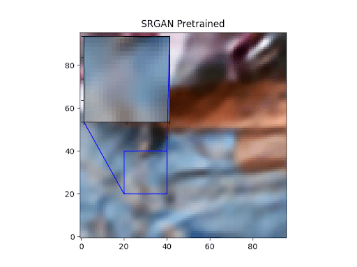
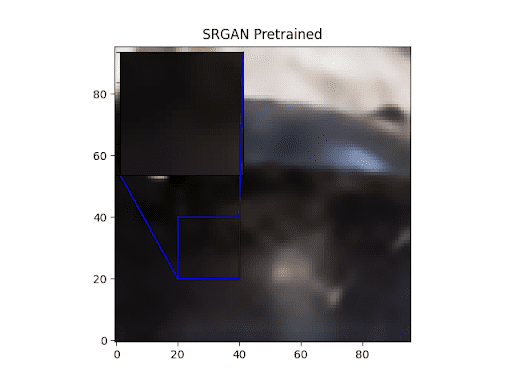
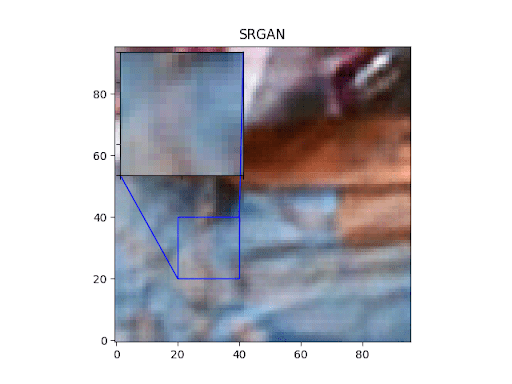
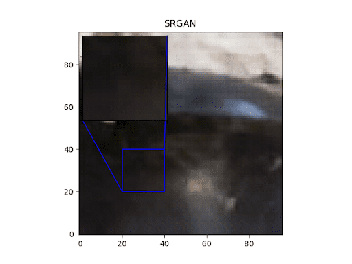
As we can clearly see, the fully trained SRGAN outputs show clearly more details than the pretrained ones.

---

---

Summary

SRGANs very smartly achieve better image super-resolution results by combining the traditional GAN elements with recipes intended to elevate visual performance.

The simple addition of the pixel-wise comparison of outputs gives us visibly stronger results when compared to previous work. However, since GANs essentially are trying to recreate data to make it look like it belongs to the training distribution, lots of computation power is necessary to achieve that. SRGANs may help you achieve your objective, but the catch is that you have to have tons of computation power ready.

---

Citation Information

Chakraborty, D. “Super-Resolution Generative Adversarial Networks (SRGAN),” PyImageSearch, P. Chugh, A. R. Gosthipaty, S. Huot, K. Kidriavsteva, R. Raha, and A. Thanki, eds., 2022, https://pyimg.co/lgnrx

@incollection{Chakraborty_2022_SRGAN,
  author = {Devjyoti Chakraborty},
  title = {Super-Resolution Generative Adversarial Networks {(SRGAN)}},
  booktitle = {PyImageSearch},
  editor = {Puneet Chugh and Aritra Roy Gosthipaty and Susan Huot and Kseniia Kidriavsteva and Ritwik Raha and Abhishek Thanki},
  year = {2022},
  note = {https://pyimg.co/lgnrx},
}

---

To download the source code to this post (and be notified when future tutorials are published here on PyImageSearch), simply enter your email address in the form below!