OpenCV Contour Approximation

In this tutorial, we’ll learn about a step-by-step implementation and utilization of OpenCV’s Contour Approximation.

When I first chanced upon the concept of Contour Approximation, the first question that hit me was: Why? Throughout my journey in Machine Learning and its related fields, I was always taught that Data is everything. Data is currency. The more you have of it, the more you are likely to succeed. Figure 1 aptly describes the scenario.

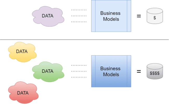
Hence, I didn’t quite understand the concept of approximating the data points of a curve. Wouldn’t that make it simpler? Wouldn’t that make us lose data? I was in for a very big surprise.

In today’s tutorial, we’ll learn about OpenCV Contour Approximation, more precisely called the Ramer–Douglas–Peucker algorithm. You’ll be amazed to know how important it was for a lot of high-priority real-life applications.

In this blog, you’ll learn:

• What Contour Approximation is
• Prerequisites required to understand Contour Approximation
• How to implement Contour Approximation
• Some Practical Applications of Contour Approximation

To learn how to implement contour approximation, just keep reading.

OpenCV Contour Approximation ( cv2.approxPolyDP )

Let’s imagine a scenario: you are a self-driving robot. You move according to the data collected by your radars (LIDAR, SONAR, etc.). You’ll constantly have to deal with tons of data that will be transformed into a format understandable to you. Then, you’ll make the decisions required for you to move. What’s your biggest obstacle in a situation like this? Is it that piece of brick purposefully left in your route? Or a zigzag road standing between you and your destination?

Turns out, the simple answer is…. All of them. Imagine the sheer amount of data you would be intaking at a given time to assess a situation. Turns out Data was playing both sides of the fence the whole time. Was Data our enemy all this time?

While it’s true that more data gives you a better perspective for your solution, it also introduces problems like computation complexity and storage. Now you, like a robot, would need to make reasonably quick decisions to traverse the route that lies in front of you.

That means simplifying complex data would be your top priority.

Let’s say you were given a top-down view of the route that you would be taking. Something like Figure 2.

What if, given the exact width of the road and other parameters, there was a way you could simplify this map? Considering your size is small enough to ignore redundant turns (parts where you can go straight without following the exact curves of the road), it would be easier for you if you could remove some redundant vertices. Something like Figure 3:

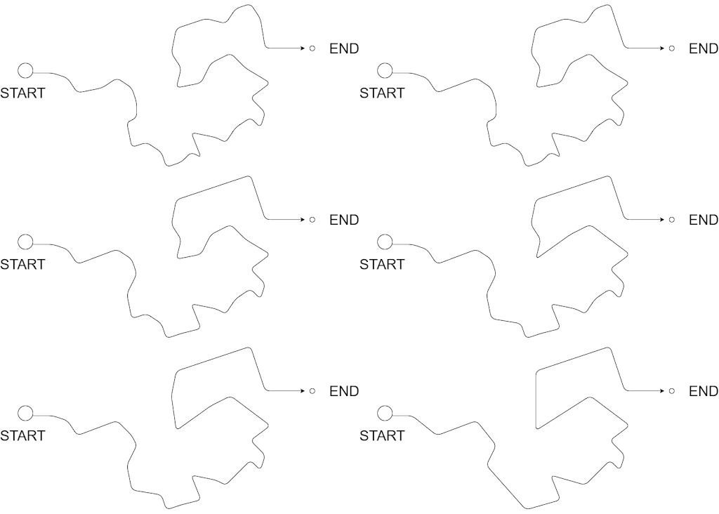
Notice how iteratively, some of the vertices are smoothened out, resulting in a much more linear route. Ingenious, isn’t it?

This is just one of the many applications Contour Approximation has in the real world. Before we proceed any further, let’s formally understand what it is.

What Is Contour Approximation?

Contour approximation, which uses the Ramer–Douglas–Peucker (RDP) algorithm, aims to simplify a polyline by reducing its vertices given a threshold value. In layman terms, we take a curve and reduce its number of vertices while retaining the bulk of its shape. For example, take a look at Figure 4.

This very informative GIF from Wikipedia’s RDP article shows us how the algorithm works. I’ll give a crude idea of the algorithm here.

Given the start and end points of a curve, the algorithm will first find the vertex at maximum distance from the line joining the two reference points. Let’s refer to it as max_point. If the max_point lies at a distance less than the threshold, we automatically neglect all the vertices between the start and end points and make the curve a straight line.

If the max_point lies outside the threshold, we’ll recursively repeat the algorithm, now making the max_point one of the references, and repeat the checking process as shown in Figure 4.

Notice how certain vertices are getting eliminated systematically. In the end, we retain the bulk of the information but in a less complex state.

With that out of the way, let’s see how we can use OpenCV to harness the power of RDP!

Configuring Your Development Environment

To follow this guide, you need to have the OpenCV library and the imutils package installed on your system.

Luckily, OpenCV is pip-installable:

$ pip install opencv-contrib-python
$ pip install imutils

If you need help configuring your development environment for OpenCV, I highly recommend that you read my pip install OpenCV guide — it will have you up and running in a matter of minutes.

Having Problems Configuring Your Development Environment?

All that said, are you:

• Short on time?
• Learning on your employer’s administratively locked system?
• Wanting to skip the hassle of fighting with the command line, package managers, and virtual environments?
• Ready to run the code right now on your Windows, macOS, or Linux system?

Then join PyImageSearch University today!

Gain access to Jupyter Notebooks for this tutorial and other PyImageSearch guides that are pre-configured to run on Google Colab’s ecosystem right in your web browser! No installation required.

And best of all, these Jupyter Notebooks will run on Windows, macOS, and Linux!

Project Structure

Let’s take a look at the project structure.

$ tree . --dirsfirst
.
├── opencv_contour_approx.py
└── shape.png

0 directories, 2 files

The parent directory contains a single script and an image:

• opencv_contour_approx.py: The only script required in the project contains all the coding involved.
• shape.png: The image on which we’ll test out Contour Approximation.

Implementing Contour Approximation with OpenCV

Before jumping to Contour Approximation, we’ll go through a few prerequisites to better understand the whole process. So, without further ado, let’s jump into opencv_contour_approx.py and start coding!

# import the necessary packages
import numpy as np
import argparse
import imutils
import cv2

# construct the argument parser and parse the arguments
ap = argparse.ArgumentParser()
ap.add_argument("-i", "--image", type=str, default="shape.png",
	help="path to input image")
args = vars(ap.parse_args())

An argument parser instance is created to give the user an easy command line interface experience when they choose the image they wish to tinker with (Lines 8-11). The default image is set as shape.png, the image which already exists in the directory. However, readers are encouraged to try this experiment out with their own custom images!

# load the image and display it
image = cv2.imread(args["image"])
cv2.imshow("Image", image)

# convert the image to grayscale and threshold it
gray = cv2.cvtColor(image, cv2.COLOR_BGR2GRAY)
thresh = cv2.threshold(gray, 200, 255,
	cv2.THRESH_BINARY_INV)[1]
cv2.imshow("Thresh", thresh)

The image provided as the argument is then read using OpenCV’s imread and displayed (Lines 14 and 15).

The image is going to look like Figure 6:

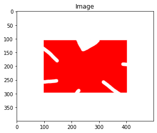
Since we’ll be using the boundary of the shape in the image, we convert the image from RGB to grayscale (Line 18). Once in grayscale format, the shape can easily be isolated using OpenCV’s threshold function (Lines 19-21). The result can be seen in Figure 7:

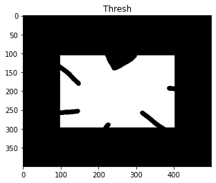
Note that since we have chosen cv2.THRESH_BINARY_INV as the parameter on Line 20, the high-intensity pixels are changed to 0, while the surrounding low-intensity pixels become 255.

# find the largest contour in the threshold image
cnts = cv2.findContours(thresh.copy(), cv2.RETR_EXTERNAL,
	cv2.CHAIN_APPROX_SIMPLE)
cnts = imutils.grab_contours(cnts)
c = max(cnts, key=cv2.contourArea)

# draw the shape of the contour on the output image, compute the
# bounding box, and display the number of points in the contour
output = image.copy()
cv2.drawContours(output, [c], -1, (0, 255, 0), 3)
(x, y, w, h) = cv2.boundingRect(c)
text = "original, num_pts={}".format(len(c))
cv2.putText(output, text, (x, y - 15), cv2.FONT_HERSHEY_SIMPLEX,
	0.9, (0, 255, 0), 2)

# show the original contour image
print("[INFO] {}".format(text))
cv2.imshow("Original Contour", output)
cv2.waitKey(0)

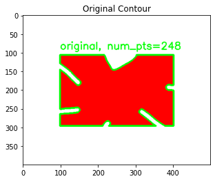
Using OpenCV’s findContours function, we can single out all possible contours in the given image (depending on the given arguments) (Lines 24 and 25). We have used the RETR_EXTERNAL argument, which only returns single representations of available contours. You can read more about it here.

The other argument used is CHAIN_APPROX_SIMPLE. This removes many vertices in a single chain line connection, vertices that are essentially redundant.

We then grab the largest contour from the array of contours (this contour belongs to the shape) and trace it on the original image (Lines 26-36). For this purpose, we use OpenCV’s drawContours function. We also use the putText function to write on the image. The output is shown in Figure 8:

Now, let’s demonstrate what contour approximation can do!

# to demonstrate the impact of contour approximation, let's loop
# over a number of epsilon sizes
for eps in np.linspace(0.001, 0.05, 10):
	# approximate the contour
	peri = cv2.arcLength(c, True)
	approx = cv2.approxPolyDP(c, eps * peri, True)

	# draw the approximated contour on the image
	output = image.copy()
	cv2.drawContours(output, [approx], -1, (0, 255, 0), 3)
	text = "eps={:.4f}, num_pts={}".format(eps, len(approx))
	cv2.putText(output, text, (x, y - 15), cv2.FONT_HERSHEY_SIMPLEX,
		0.9, (0, 255, 0), 2)

	# show the approximated contour image
	print("[INFO] {}".format(text))
	cv2.imshow("Approximated Contour", output)
	cv2.waitKey(0)

As mentioned earlier, we’ll need a value eps, which will act as the threshold value to measure vertices. Accordingly, we start looping epsilon’s (eps) value over a range to feed it to the contour approximation function (Line 45).

On Line 47, the perimeter of the contour is calculated using cv2.arcLength. We then use the cv2.approxPolyDP function and initiate the contour approximation process (Line 48). The eps × peri value acts as the approximation accuracy and will change with each epoch due to eps’s incremental nature.

We proceed to trace the resultant contour on the image on each epoch to assess the results (Lines 51-60).

Let’s see the results!

Contour Approximation Results

Before moving on to the visualizations, let’s see how contour approximation affected the values.

$ python opencv_contour_approx.py
[INFO] original, num_pts=248
[INFO] eps=0.0010, num_pts=43
[INFO] eps=0.0064, num_pts=24
[INFO] eps=0.0119, num_pts=17
[INFO] eps=0.0173, num_pts=12
[INFO] eps=0.0228, num_pts=11
[INFO] eps=0.0282, num_pts=10
[INFO] eps=0.0337, num_pts=7
[INFO] eps=0.0391, num_pts=4
[INFO] eps=0.0446, num_pts=4
[INFO] eps=0.0500, num_pts=4

Notice how, with each increasing value of eps, the number of points in the contour keeps decreasing? This signifies that the approximation did indeed work. Note that at an eps value of 0.0391, the number of points starts to saturate. Let’s analyze this better with visualizations.

Contour Approximation Visualizations

Through Figures 9-12, we chronicle the evolution of the contour through some of the epochs.

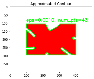
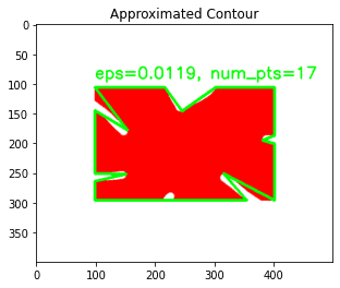
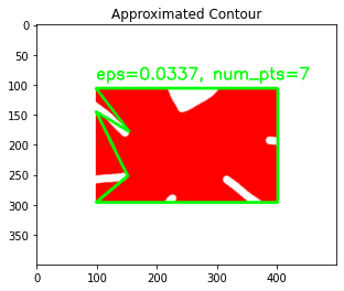
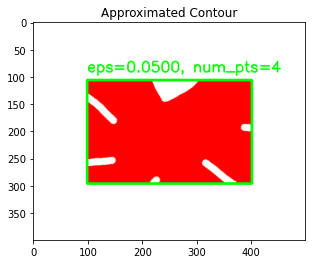
Notice how gradually the curves get smoother and smoother. As the threshold increases, the more linear it gets. By the time the value of eps has reached 0.0500, the contour is now a perfect rectangle, having a mere 4 points. That’s the power of the Ramer–Douglas–Peucker algorithm.

Credits

Distorted shape image inspired by OpenCV documentation.

Summary

Simplifying data while retaining the bulk of the information is probably one of the most sought-after scenarios in this data-driven world. Today, we learned about how RDP is used to simplify our tasks. Its contribution to the vector graphics and robotics field is immense.

RDP also spreads over to other domains like Range Scanning, where it is used as a denoising tool. I hope this tutorial helped you understand how you can use contour approximation in your work.

Citation Information

Chakraborty, D. “OpenCV Contour Approximation ( cv2.approxPolyDP ),” PyImageSearch, 2021, https://pyimagesearch.com/2021/10/06/opencv-contour-approximation/ 

@article{dev2021opencv, author = {Devjyoti Chakraborty}, title = {Open{CV} Contour Approximation ( cv2.approx{PolyDP} )}, journal = {PyImageSearch}, year = {2021}, note = {https://pyimagesearch.com/2021/10/06/opencv-contour-approximation/}, }

To download the source code to this post (and be notified when future tutorials are published here on PyImageSearch), simply enter your email address in the form below!