Table of Contents
- What’s Behind PyTorch 2.0? TorchDynamo and TorchInductor (primarily for developers)
- Technology Behind PyTorch 2.0
- TorchDynamo
- TorchInductor
- AOT Autograd
- PrimTorch
- Configuring Your Development Environment
- Installation
- Verification
- Need Help Configuring Your Development Environment?
- Project Structure
- Accelerating DNNs Using TorchDynamo
- TorchDynamo vs. TorchScript vs. FX Tracing
- Data-Dependent Control Flow
- Non-PyTorch Libraries
- TorchDynamo FX Graphs
- Summary
What’s Behind PyTorch 2.0? TorchDynamo and TorchInductor (primarily for developers)
In our previous lesson of this series, we saw how PyTorch 2.0’s new feature, torch.compile, can provide significant speedups of 30-200% in eager mode for most models we run daily. PyTorch 2.0 introduces the following new technologies:
- TorchDynamo
- TorchInductor
- AOT Autograd
- PrimTorch
These technologies make the PyTorch 2.0 code run faster (with less memory) by JIT-compiling the PyTorch 2.0 code into optimized kernels, all while requiring minimal code changes.
This lesson covers these technologies in more detail and digs deeper into the usage and behavior of both TorchDynamo and TorchInductor. We will see how we can accelerate our models just like torch.compile but using TorchDynamo/TorchInductor and demonstrate some of the advantages of both TorchDynamo and TorchInductor over previous compiler solutions like TorchScript and FX (Function eXtraction) Tracing. This tutorial is primarily for developers who want to accelerate their deep learning models with PyTorch 2.0.
In this series, you will learn about Accelerating Deep Learning Models with PyTorch 2.0.
This lesson is the 2nd of a 2-part series on Accelerating Deep Learning Models with PyTorch 2.0:
- What’s New in PyTorch 2.0?
torch.compile - What’s Behind PyTorch 2.0? TorchDynamo and TorchInductor (primarily for developers) (this tutorial)
To learn what’s behind PyTorch 2.0, just keep reading.
What’s Behind PyTorch 2.0? TorchDynamo and TorchInductor (primarily for developers)
We will start with understanding the new technologies behind PyTorch 2.0.
Technology Behind PyTorch 2.0
TorchDynamo
TorchDynamo (shown in Figure 1) is PyTorch’s latest compiler solution that leverages JIT (Just In Time) compilation to transform a general Python program into an FX Graph. The FX Graph is an intermediate representation of your code that can be further compiled and optimized. TorchDynamo extracts FX Graphs by inspecting Python bytecode at runtime and detecting calls to PyTorch operations.

Additionally, TorchDynamo is designed to mix Python execution with compiled backends to get the best of both worlds: usability and performance. Finally, it can support the arbitrary program by breaking the FX Graph whenever it encounters any unsupported feature (e.g., data-dependent flows or non-PyTorch libraries).
The approach is based on a CPython feature known as Frame Evaluation API that can safely and correctly capture graphs 99% of the time without incurring additional overhead. Other previous compiler solutions like TorchScript and FX Tracing need help to capture graphs even 50% of the time, and that too with additional overhead.
Here’s how TorchDynamo’s behavior differs from the default Python behavior.
TorchInductor
TorchDynamo should be paired with a backend that can efficiently convert captured FX Graphs into fast machine code to make PyTorch 2.0 programs faster. However, a lot is lost while exporting the FX Graphs in different existing backends. Some have fundamentally different execution models than PyTorch, and others are only optimized for inference and not training.
TorchInductor is the new compiler backend that compiles the FX Graphs generated by TorchDynamo into optimized C++/Triton kernels. TorchInductor uses a Pythonic define-by-run loop level intermediate representation to automatically map PyTorch models into generated Triton code on GPUs and C++/OpenMP on CPUs. TorchInductor’s core loop level intermediate representation contains only ~50 operators, and it is implemented in Python, making it easily hackable and extensible.
AOT Autograd
AOT Autograd is PyTorch’s new automatic differentiation engine that leverages PyTorch’s torch_dispatch mechanism to trace through the autograd engine and create ahead-of-time backward passes. This accelerates both forward and backward passes.
PrimTorch
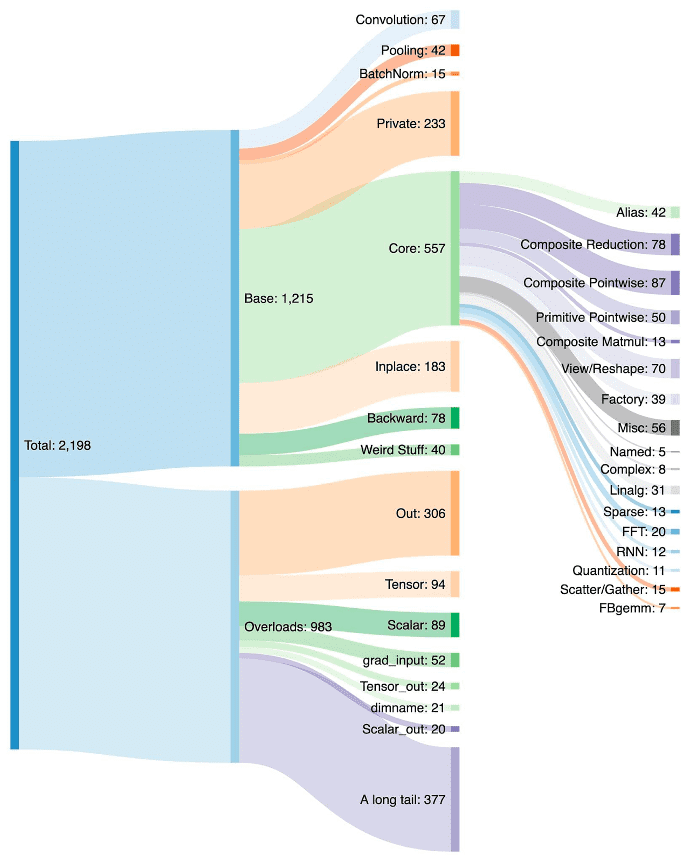
With more than 2000+ operators, writing a backend for PyTorch is challenging and draining. Hence, with PrimTorch (Figure 2), PyTorch 2.0 canonicalizes these operations into smaller primitive operations. As a result, there are mainly two operation sets in PrimTorch:
- Prim ops: contain
~250low-level operations are well suited for compilers and can be fused for good performance. - ATen ops: contain
~750canonical operators suited for backends that won’t have a compilation to recover performance from a lower-level operator set like Prim ops.
Configuring Your Development Environment
Installation
As in previous versions, PyTorch 2.0 is available as a Python pip package. However, to successfully install PyTorch 2.0, your system should have installed the latest CUDA (Compute Unified Device Architecture) versions (11.6 and 11.7). Here’s how you can install PyTorch 2.0 nightly version via pip:
For CUDA version 11.7:
$ pip3 install numpy --pre torch --force-reinstall --extra-index-url https://download.pytorch.org/whl/nightly/cu117
For CUDA version 11.6:
$ pip3 install numpy --pre torch --force-reinstall --extra-index-url https://download.pytorch.org/whl/nightly/cu116
However, if you don’t have CUDA 11.6 or 11.7 installed on your system, you can download all the required dependencies in the PyTorch nightly binaries with docker.
$ sudo apt install -y nvidia-docker2
$ sudo systemctl restart docker
$ docker pull ghcr.io/pytorch/pytorch-nightly
$ docker run --gpus all -it ghcr.io/pytorch/pytorch-nightly:latest /bin/bash
Be sure to specify --gpus all so your container can access all your GPUs.
Verification
Optionally, you can verify your installation via:
$ git clone https://github.com/pytorch/pytorch
$ cd tools/dynamo
$ python verify_dynamo.py
Also, ensure you have a C++ compiler installed. You can install the g++ compiler via:
$ sudo apt-get install g++
Need Help Configuring Your Development Environment?
All that said, are you:
- Short on time?
- Learning on your employer’s administratively locked system?
- Wanting to skip the hassle of fighting with the command line, package managers, and virtual environments?
- Ready to run the code immediately on your Windows, macOS, or Linux system?
Then join PyImageSearch University today!
Gain access to Jupyter Notebooks for this tutorial and other PyImageSearch guides pre-configured to run on Google Colab’s ecosystem right in your web browser! No installation required.
And best of all, these Jupyter Notebooks will run on Windows, macOS, and Linux!
Project Structure
We first need to review our project directory structure.
Start by accessing the “Downloads” section of this tutorial to retrieve the source code.
From there, take a look at the directory structure:
├── dynamo_speedup.py
├── data_dependent_cf.py
├── non_pytorch_function.py
├── dynamo_graph.py
The project directory contains four files.
- First, the
dynamo_speedup.pyfile demonstrates how to achieve speedups on real models using both TorchDynamo and TorchInductor. - Next, the file
data_dependent_cf.pyandnon_pytorch_function.pydemonstrates the advantages of TorchDynamo over existing compiler solutions like TorchScript and FX Tracing. - Finally, the file
dynamo_graph.pyshows how we can analyze and view graphs and graph breaks created by TorchDynamo. We will discuss these files in detail in subsequent sections.
Accelerating DNNs Using TorchDynamo
We will start our hands-on exercise by looking at speeding up deep neural networks (DNNs) like torch.compile but using TorchDynamo. First, look into the dynamo_speedup.py file in the project directory.
import torch
import torch._dynamo as dynamo
import time
import numpy as np

# running a model
def run_model(model, inputs, steps=20):
    # load model on GPU
    model = model.cuda()
    # define an optimizer
    optimizer = torch.optim.Adam(model.parameters())
    times = []
    for step in range(steps):
        begin = time.time()
        # zero gradients
        optimizer.zero_grad()
        # forward pass
        output = model(inputs.cuda())
        # back propagate
        output.sum().backward()
        # optimize weights
        optimizer.step()
        end = time.time()
        # calculate step time
        times.append(float(end - begin))
        print(f"Time for {step}-th forward pass is {end - begin}")

    # calculate median step time
    median = np.median(times)
    print("Median step time is {:.3f} seconds".format(median))
    return median
On Lines 1-4, we import the torch, numpy, and time libraries. Next, we import the TorchDynamo engine from torch._dynamo. Then on Lines 7-31, we define the run_model() function that takes model, inputs, and steps as arguments and runs the model training on inputs for a given number of steps. First, on Line 9, we load the model on the GPU. Then on Line 11, we define optimizer over model parameters.
Finally, on Lines 13-26, we run the model training for given steps wherein we pass the given inputs, backpropagate gradients, and update network weights in each step. We print and store the time taken by each step in a list of times. Finally, on Lines 29 and 30, we calculate and print the median step time taken by our compiled model.
# loading pretrained resnet50
model = torch.hub.load('pytorch/vision:v0.10.0', "resnet50", pretrained=True)
# random input image
inputs = torch.randn(256, 3, 224, 224)

# run original model
print("Running Original ResNet50...")
time1 = run_model(model, inputs, 10)

# optimize model using dynamo
optimized_model = dynamo.optimize("inductor")(model)
# run optimized model
print("Running Optimized ResNet50...")
time2 = run_model(optimized_model, inputs, 10)

#calculate training speedup
print("Speedup : {:.3f}%".format(100*(time1-time2)/time1))
Next, on Lines 34-36, we load a pre-trained ResNet50 model using torch.hub and define a dummy input image inputs with batch size 256. On Line 40, we run the original model and calculate its median step time. Then on Line 43, we optimize the model with dynamo.optimize() using the inductor backend. This function is analogous to torch.compile and is expected to provide similar results. Next, on Line 46, we run the optimized_model and calculate its median step time. Finally, on Line 49, we calculate the speedup given by optimized_model over the original model.
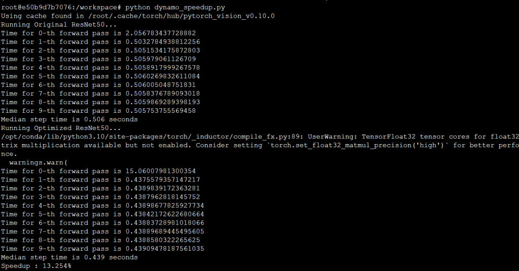
After running the above script using python dynamo_speedup.py, your output should look similar to Figure 3.
By using TorchDynamo, we can achieve a 13% speedup for ResNet50. Note that your numbers differ slightly depending on your hardware accelerator. This experiment is done on NVIDIA A6000s. Newer GPUs like A100s are likely to provide more speedups.
Also, notice that TorchDynamo and TorchInductor take much longer to complete in eager mode at the first step. This is because TorchDynamo and TorchInductor compile the model into optimized kernels as it executes.
TorchDynamo vs. TorchScript vs. FX Tracing
Now that we have seen that TorchDynamo can provide speedup for real models, it is important to understand in what other aspects it is better than previous compiler solutions like TorchScript and FX Tracing. The primary advantage of TorchDynamo lies in its ability to handle arbitrary Python code without significant changes. In this section, we will discuss these advantages in detail.
Data-Dependent Control Flow
Data-dependent control flows are one case that TorchDynamo can handle that other compilers fail to capture. Data-dependent control flow means that the flow of data depends on the value of the data itself. The file data_dependent_cf.py in the project directory illustrates this concept.
import torch
import torch._dynamo as dynamo
import torch.jit as jit
import torch.fx as fx
import traceback as tb
import warnings
warnings.simplefilter("ignore", UserWarning)

# define a function with data-dependent control flow
def f1(x):
    if x.sum() < 0:
        return torch.tensor(0)
    return torch.tensor(1)

# Check if output of two functions is same for given input
# fn1 is the original function
# fn2 is the compiled function
def test_fns(f1, f2, x):
    out1 = f1(x)
    out2 = f2(x)
    return torch.allclose(out1, out2)
On Lines 1-6, we import standard libraries and packages like torch, TorchDynamo torch._dynamo, TorchScript torch.jit, and FX Tracing torch.fx. Next, on Lines 10-13, we define a function f1() that takes a PyTorch tensor x and returns 0 or 1 depending on the polarity of its sum. Here, Line 11 (i.e., if x.sum() < 0:) is an example of data-dependent control flow.
Then on Lines 18-21, we define a function test_fns that takes two functions, f1 and f2, as arguments along with an input x to check whether both functions return the same output for the same set of input x. This function will tell us whether our original or compiled function has the same behavior.
# define random input
x = torch.randn(5, 5)

# compile using TorchScipt
traced_f1 = jit.trace(f1, (x,))
# compare f1, and traced_f1 on -x
print("TorchScript:", test_fns(f1, traced_f1, (-x)))

# compile using FX
fx_f1 = fx.symbolic_trace(f1, concrete_args={"x": x})
# compare f1, and fx_f1 on -x
print("FX:", test_fns(f1, fx_f1, (-x)))

# compile using Dynamo
dynamo_f1 = dynamo.optimize("inductor")(f1)
# compare f1, and dynamo_f1 on -x
print("TorchDynamo:", test_fns(f1, dynamo_f1, (-x)))
Next, on Line 24, we define a dummy input x. On Line 27, we compile the function f1 using TorchScript jit.trace(f1, (x,)) that takes the original function f1 and a dummy input x. On Line 29, we compare the compiled model traced_f1 and the original function f1 on -x instead of x.
On Line 32, we compile the function f1 using FX Tracing fx.symbolic_trace(f1, concrete_args={"x": x}) that also takes the original function f1 and a dummy input x. On Line 34, we compare the compiled model fx_f1 and the original function f1 on -x instead of x.
Finally, on Line 37, we compile the function f1 using TorchDynamo dynamo.optimize("inductor")(f1) that takes the original function f1 as input. Then, on Line 39, we compare the compiled model dynamo_f1 and the original function f1 on -x.
After running the script python data_dependent_cf.py, your output should look like Figure 4.

As you can see from the above output, TorchScript and FX Tracing fails to correctly capture the behavior of our function when a data-dependent control flow is present. This is because these solutions only capture or trace the path taken by the provided dummy input, which is x in our case. However, when we flip the input to -x, they follow the same old traced path and yield the wrong result.
TorchDynamo, however, correctly captures the function and yields the correct result. It does so by breaking the computation graph whenever it encounters a data-dependent control flow and letting the Python interpreter handle the unsupported code and resume graph capturing afterward.
Non-PyTorch Libraries
Another case where TorchDynamo has an advantage over TorchScript and FX Tracing is when the program contains non-PyTorch functions. The file non_pytorch_function.py in the project directory illustrates this use case. For this example, you need to install scipy, which you can install via pip install scipy.
import torch
import torch._dynamo as dynamo
import torch.jit as jit
import torch.fx as fx
import traceback as tb
import scipy
import warnings
warnings.simplefilter("ignore", UserWarning)

# define a function with non-PyTorch library
def f1(x):
    x = x * 2
    x = scipy.fft.dct(x.numpy())
    x = torch.from_numpy(x)
    x = x * 2
    return x

# Check if output of two functions is same for given input
# fn1 is the original function
# fn2 is the compiled function
def test_fns(f1, f2, x):
    out1 = f1(x)
    out2 = f2(x)
    return torch.allclose(out1, out2)

# define random input
x = torch.randn(5, 5)

# compile using TorchScipt
traced_f1 = jit.trace(f1, (x,))
# compare f1, and traced_f1 on -x
print("TorchScript:", test_fns(f1, traced_f1, (-x)))

# compile using FX
fx_f1 = fx.symbolic_trace(f1, concrete_args={"x": x})
# compare f1, and fx_f1 on -x
print("FX:", test_fns(f1, fx_f1, (-x)))

# compile using Dynamo
dynamo_f1 = dynamo.optimize("inductor")(f1)
# compare f1, and dynamo_f1 on -x
print("TorchDynamo:", test_fns(f1, dynamo_f1, (-x)))
On Lines 1-7, we import standard libraries and packages like torch, scipy, TorchDynamo torch._dynamo, TorchScript torch.jit, and FX Tracing torch.fx. Next, on Lines 11-16, we define a function f1() that takes a PyTorch tensor x and operates on it using functions from the scipy package. Note that scipy.fft.dct() is a non-PyTorch function. The rest of the code (Lines 21-42) is the same as in the previous example.
After running the script python non_pytorch_function.py, your output should look like Figure 5.

As with the previous example, we can see that TorchScript and FX Tracing fail whenever they encounter any non-PyTorch code. This is because these solutions treat output from non-PyTorch functions as constants in the computation graph which can silently yield wrong results.
TorchDynamo successfully captures the graph even when non-Pytorch functions are used.
It should be noted that it’s different from TorchScript or FX Tracing and cannot handle data-dependent control flows or non-PyTorch functions. They can handle these cases; however, the solution can require significant code changes and will raise errors when unsupported Python is used.
TorchDynamo FX Graphs
We will now understand how we can analyze the FX Graphs captured by TorchDynamo, along with graph breaks. Generally, TorchDynamo captures an arbitrary Python code and converts it into an FX Graph, which TorchInductor then consumes to yield optimized kernels. Hence, TorchDynamo can work even with other backends. First, however, we will implement our custom backend to analyze the FX Graphs. We will refer to the dynamo_graph.py file in our project directory for this demo.
import torch
import torch._dynamo as dynamo
from typing import List

# define a custom backend to print FX graph
def custom_backend(gm: torch.fx.GraphModule, example_inputs: List[torch.Tensor]):
    print("custom backend called with FX graph:")
    gm.graph.print_tabular()
    return gm.forward

# Reset since we are using a different backend (a custom one).
dynamo.reset()

# define a function with data-dependent control flow
def f1(x, y):
    z = torch.nn.functional.sigmoid(y)
    if x.sum() < 0:
        x = x*-1
    return z*x

x, y = torch.randn(10), torch.randn(10)

explanation, out_guards, graphs, ops_per_graph, break_reasons, explanation_verbose = dynamo.explain(f1, x, y)
print(explanation_verbose)
for graph in graphs:
    print(graph.graph.print_tabular())
On Lines 1-3, we import the torch and torch._dynamo packages. Then on Lines 6 and 7, we implement our custom_backend() function that takes an FX Graph instance gm and a list of input tensors example_inputs and prints the computation graph. On Line 12, we subsequently reset the dynamo engine to use our custom backend. Next, on Lines 15-19, we implement a function f1 ( with data-dependent control flow) that takes two inputs, x and y, and returns an output based on the polarity of x.sum().
On Line 21, we define dummy inputs. Then, on Lines 23-26, we use dynamo.explain to print the graphs and graph breaks in the code.
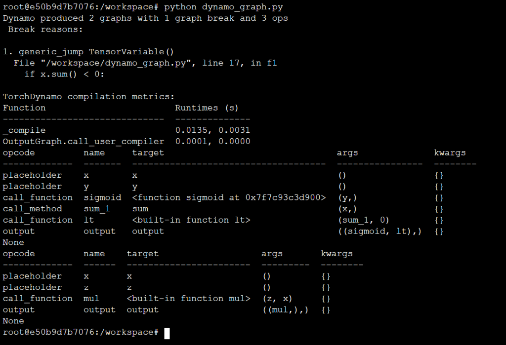
After running the script python dynamo_graph.py, you will see the following output on your console (Figure 6).
From Figure 6, we can see that TorchDynamo extracts two graphs from the code corresponding to graph break at the statement if x.sum() < 0: x = -x.
- Graph 1:
z = torch.nn.functional.sigmoid(y); x = x*-1; z*x - Graph 2:
z = torch.nn.functional.sigmoid(y); z*x
So whenever x.sum() < 0, dynamo executes Graph 1, i.e., evaluates the first statement y = torch.nn.functional.sigmoid(y) and then lets the Python interpreter evaluate the conditional statement and then runs statement return y*x. However, when x.sum() >= 0, dynamo executes Graph 2 where it first evaluates y = torch.nn.functional.sigmoid(y) and then lets the Python interpreter evaluate the conditional statement and then run statement return y*x.
This highlights a significant difference between TorchDynamo and previous PyTorch compiler solutions. When encountering unsupported Python features, previous solutions either raise an error or silently fail. TorchDynamo, on the other hand, will break the computation graph.
What's next? We recommend PyImageSearch University.
86+ total classes • 115+ hours hours of on-demand code walkthrough videos • Last updated: March 2026
★★★★★ 4.84 (128 Ratings) • 16,000+ Students Enrolled
I strongly believe that if you had the right teacher you could master computer vision and deep learning.
Do you think learning computer vision and deep learning has to be time-consuming, overwhelming, and complicated? Or has to involve complex mathematics and equations? Or requires a degree in computer science?
That’s not the case.
All you need to master computer vision and deep learning is for someone to explain things to you in simple, intuitive terms. And that’s exactly what I do. My mission is to change education and how complex Artificial Intelligence topics are taught.
If you're serious about learning computer vision, your next stop should be PyImageSearch University, the most comprehensive computer vision, deep learning, and OpenCV course online today. Here you’ll learn how to successfully and confidently apply computer vision to your work, research, and projects. Join me in computer vision mastery.
Inside PyImageSearch University you'll find:
- ✓ 86+ courses on essential computer vision, deep learning, and OpenCV topics
- ✓ 86 Certificates of Completion
- ✓ 115+ hours hours of on-demand video
- ✓ Brand new courses released regularly, ensuring you can keep up with state-of-the-art techniques
- ✓ Pre-configured Jupyter Notebooks in Google Colab
- ✓ Run all code examples in your web browser — works on Windows, macOS, and Linux (no dev environment configuration required!)
- ✓ Access to centralized code repos for all 540+ tutorials on PyImageSearch
- ✓ Easy one-click downloads for code, datasets, pre-trained models, etc.
- ✓ Access on mobile, laptop, desktop, etc.
Summary
TorchDynamo and TorchInductor are the primary technologies that power PyTorch 2.0. TorchInductor is capable of safely and correctly capturing/generating computation graphs from arbitrary Python code without significant changes in the code. TorchInductor, on the other hand, takes the computation graph generated by TorchDynamo and converts it into optimized low-level kernels.
By using dynamo.optimize(), one can speed up real deep learning models up to 13% on NVIDIA A6000s. Furthermore, TorchDynamo outperforms existing solutions like TorchScript and FX Tracing by handling data-dependent control flows and non-PyTorch code without any significant changes to the code. It does so by breaking the computation graph whenever encountering an unsupported feature. It also allows the Python interpreter to handle the unsupported code and resume graph capturing afterward.
Citation Information
Mangla, P. “What’s Behind PyTorch 2.0? TorchDynamo and TorchInductor (primarily for developers),” PyImageSearch, P. Chugh, A. R. Gosthipaty, S. Huot, K. Kidriavsteva, R. Raha, and A. Thanki, eds., 2023, https://pyimg.co/u6xmk
@incollection{Mangla_2023_PT2TDTI4dev,
  author = {Puneet Mangla},
  title = {What's Behind {PyTorch} 2.0? {TorchDynamo} and {TorchInductor} (primarily for developers)},
  booktitle = {PyImageSearch}},
  editor = {Puneet Chugh and Aritra Roy Gosthipaty and Susan Huot and Kseniia Kidriavsteva and Ritwik Raha and Abhishek Thanki},
  year = {2023},
  url = {https://pyimg.co/u6xmk},
}

Unleash the potential of computer vision with Roboflow - Free!
- Step into the realm of the future by signing up or logging into your Roboflow account. Unlock a wealth of innovative dataset libraries and revolutionize your computer vision operations.
- Jumpstart your journey by choosing from our broad array of datasets, or benefit from PyimageSearch’s comprehensive library, crafted to cater to a wide range of requirements.
- Transfer your data to Roboflow in any of the 40+ compatible formats. Leverage cutting-edge model architectures for training, and deploy seamlessly across diverse platforms, including API, NVIDIA, browser, iOS, and beyond. Integrate our platform effortlessly with your applications or your favorite third-party tools.
- Equip yourself with the ability to train a potent computer vision model in a mere afternoon. With a few images, you can import data from any source via API, annotate images using our superior cloud-hosted tool, kickstart model training with a single click, and deploy the model via a hosted API endpoint. Tailor your process by opting for a code-centric approach, leveraging our intuitive, cloud-based UI, or combining both to fit your unique needs.
- Embark on your journey today with absolutely no credit card required. Step into the future with Roboflow.
To download the source code to this post (and be notified when future tutorials are published here on PyImageSearch), simply enter your email address in the form below!

Download the Source Code and FREE 17-page Resource Guide
Enter your email address below to get a .zip of the code and a FREE 17-page Resource Guide on Computer Vision, OpenCV, and Deep Learning. Inside you'll find my hand-picked tutorials, books, courses, and libraries to help you master CV and DL!


Comment section
Hey, Adrian Rosebrock here, author and creator of PyImageSearch. While I love hearing from readers, a couple years ago I made the tough decision to no longer offer 1:1 help over blog post comments.
At the time I was receiving 200+ emails per day and another 100+ blog post comments. I simply did not have the time to moderate and respond to them all, and the sheer volume of requests was taking a toll on me.
Instead, my goal is to do the most good for the computer vision, deep learning, and OpenCV community at large by focusing my time on authoring high-quality blog posts, tutorials, and books/courses.
If you need help learning computer vision and deep learning, I suggest you refer to my full catalog of books and courses — they have helped tens of thousands of developers, students, and researchers just like yourself learn Computer Vision, Deep Learning, and OpenCV.
Click here to browse my full catalog.