Learning JAX in 2023: Part 3 — A Step-by-Step Guide to Training Your First Machine Learning Model with JAX

---

---

Table of Contents

---

Learning JAX in 2023: Part 3 — A Step-by-Step Guide to Training Your First Machine Learning Model with JAX

In this tutorial, you will learn how to train your first machine learning model with JAX.

This lesson is the last of a 3-part series on Learning JAX in 2023:

1. Learning JAX in 2023 | Part 1 — The Ultimate Guide to Accelerating Numerical Computation and Machine Learning
2. Learning JAX in 2023 | Part 2 — JAX’s Power Tools grad, jit, vmap, and pmap
3. Learning JAX in 2023: Part 3 — A Step-by-Step Guide to Training Your First Machine Learning Model with JAX (this tutorial)

To learn how to train your first machine learning model with JAX and PyTrees, just keep reading.

---

Learning JAX in 2023: Part 3 — A Step-by-Step Guide to Training Your First Machine Learning Model with JAX

We conclude our “Learning JAX in 2023” series with a hands-on tutorial. Throughout the series, we have covered the theoretical concepts of JAX, and in this post, we will apply those concepts to train a machine learning model. By the end of this tutorial, you will have a solid understanding of how to train a machine learning model using JAX and will be able to apply this knowledge to other ML problems.

The PyImageSearch team is dedicated to providing readers with the resources to better understand machine learning concepts through code. We will put everything we learned so far into gradually building a multilayer perceptron (MLP) with PyTrees. We have slowly broken down the tutorial into bits and pieces to present new concepts.

We hope this post will be a valuable resource as you continue learning and exploring the world of JAX.

---

Configuring Your Development Environment

To follow this guide, you need to have the JAX library installed on your system.

Luckily, JAX is pip-installable:

$ pip install jax

---

Having Problems Configuring Your Development Environment?

All that said, are you:

• Short on time?
• Learning on your employer’s administratively locked system?
• Wanting to skip the hassle of fighting with the command line, package managers, and virtual environments?
• Ready to run the code on your Windows, macOS, or Linux system now?

Then join PyImageSearch University today!

Gain access to Jupyter Notebooks for this tutorial and other PyImageSearch guides that are pre-configured to run on Google Colab’s ecosystem right in your web browser! No installation required.

And best of all, these Jupyter Notebooks will run on Windows, macOS, and Linux!

---

🚝 Train a Simple Model with JAX

In this section, we will construct two basic models. The first model comprises a single weight and bias, whereas the second model has two weights and two biases.

But will they be able to learn? Of course, they will. We will first create and model a linear dataset using our linear model. Next, we will introduce nonlinearity using various activation functions.

The gradual increase in complexity will not only assist us in understanding the concepts better but also make it easier to implement code using JAX.

Before we build models using JAX, we first need to acquire a dataset. A simple one will suffice, as our goal is to demonstrate how to build models using JAX.

---

Build a Linear Dataset

Let us build a linear dataset. We will take the help of the well-known equation of a line to produce our data:

where is the dependent variable, is the independent variable, is the slope of the line, and is the -intercept of the line.

# Build the PRNG key
key = jax.random.PRNGKey(42)

xs = random.normal(key, shape=(128, 1))

# Hyperparameters for the linear function
m = 2.0
c = 4.0

# Build the linear function
ys = (m*xs) + c

We create a pseudorandom number generator (PRNG) key with the value of 42, which is used to seed the random number generation.

The normal function from the random module of JAX generates an array of 128 random values with a shape of (128, 1), where each value is sampled from a normal distribution.

Then we define the hyperparameters for the linear function.

The hyperparameters define the linear function, where xs is the array of random values, and ys is the resulting array of values computed by the linear function.

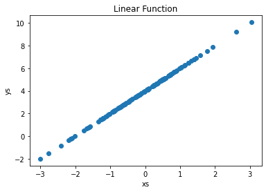
Figure 1 visualizes the linear function using matplotlib.

# Visualizing the function
plt.scatter(xs, ys)
plt.xlabel("xs")
plt.ylabel("ys")
plt.title("Linear Function")
plt.show()

---

Linear Model

Now that our linear function is ready to be modeled, let’s start creating our first machine learning model.

To combat a linear dataset, we build a linear regression model. The model will consist of a single weight and a single bias parameter that will be learned.

def linear_model(theta, x):
    """
    The linear model that will fit on the linear function.

    Args:
        - theta: Collection of weights and biases.
        - x: The input to the model.
    
    Returns:
        The prediction from the model.
    """
    weight, bias = theta
    pred = x * weight + bias
    return pred

The linear_model function is a simple linear model that takes in an input x and a collection of parameters called theta (which is a tuple of weight and bias) and returns a prediction based on the linear equation y = x * weight + bias.

def get_loss(theta, x, y):
    """
    The loss function. We use the L2 distance as our loss function.

    Args:
        - theta: Parameters of the model.
        - x: Input to the model.
        - y: The ground truth of the dataset.
    
    Returns:
        A scalar loss between the ground truth and the predicted value.
    """
    pred = linear_model(theta, x)
    loss = jnp.mean((y - pred)**2)
    return loss

The loss function is used to compute the loss of a linear model based on the following:

• input x
• ground truth y
• model’s parameters theta

It first calls the linear_model function, passing in theta and x as arguments to get the predicted output of the linear model. Then it calculates the loss between the predicted output and the ground truth y using the mean squared error (MSE) as a loss function.

@jit
def update_step(theta, x, y, lr):
    """
    A single update step for our model. We use the simple stochastic
    gradient update as our optimizer.

    Args:
        - theta: Parameters of the model.
        - x: Input to the model.
        - y: The ground truth of the dataset.
        - lr: Learning rate of the optimizer.
    
    Returns:
        - The current updated state of the model parameters.
        - The current loss
    """
    loss, gradient = value_and_grad(get_loss)(theta, x, y)
    updated_theta = theta - lr * gradient
    return updated_theta, loss

The update_step function performs a single update step (as the name suggests) on the linear model’s parameters theta, using the input x and the ground truth y, and the learning rate lr.

It uses the jax.value_and_grad function from the JAX library, which takes a function as an argument and returns the value of the function and its gradient with respect to its inputs.

Then we calculate the loss and its gradient by calling the get_loss function with theta, x, and y.

We update the parameters theta by subtracting the product of the learning rate lr and the gradient from the current value of theta.

# Initialize the parameters of the model
weight = 0.0
bias = 0.0
theta = jnp.array([weight, bias])

Here, we initialize the model. The parameters of the model are initialized with zeros. We encourage you to try other initialization techniques as well.

# Iterate and update the parameters
epochs = 10000
for iter in range(epochs):
    theta, loss = update_step(theta, xs, ys, 1e-4)
    if iter % 1000 == 0 and iter != 0:
        print(f"ITER {iter} | LOSS {loss:.4f}")

Finally, we train our linear model using stochastic gradient descent.

Each loop iteration calls the update_step function with the current parameters theta, the input xs, the ground truth ys, and a learning rate of 1e-4. The update_step function returns the updated parameters and the current loss of the model.

The updated parameters and the current loss are then assigned to the variables theta and loss, respectively. The final value of theta obtained from the loop will be the trained parameters of the model that can be used to make predictions on new data.

>>> ITER 1000 | LOSS 12.5518
>>> ITER 2000 | LOSS 8.7530
>>> ITER 3000 | LOSS 6.1060
>>> ITER 4000 | LOSS 4.2608
>>> ITER 5000 | LOSS 2.9740
>>> ITER 6000 | LOSS 2.0763
>>> ITER 7000 | LOSS 1.4499
>>> ITER 8000 | LOSS 1.0126
>>> ITER 9000 | LOSS 0.7074

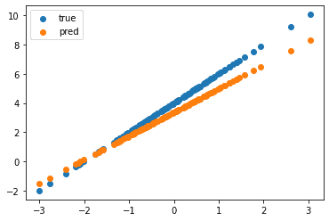
Once we have our model trained, let’s see how it did on the training dataset. From Figure 2, we can see that the model fits the dataset quite well.

plt.scatter(xs, ys, label="true")
plt.scatter(xs, linear_model(theta, xs), label="pred")
plt.legend()
plt.show()

---

Build a Nonlinear Dataset

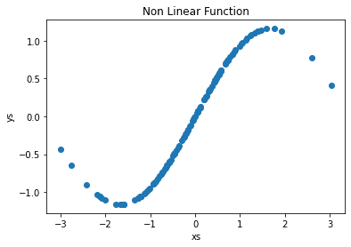
Let’s take this implementation up a notch. What do we do if our data comes from a nonlinear distribution? The linear regression model does not work anymore. We have to include some nonlinearity into the model now!

# Build the dataset
xs = random.normal(key, shape=(128, 1))

mu = 0.0
sigma = 0.1
noise = mu + sigma * random.normal(key, shape=(128, 1))

ys = jnp.sin(xs) + noise

We generate xs the same way as shown above.

We define the parameters for a Gaussian noise that we will add to the xs values to create the ground truth ys for the model.

We set the following:

• mu: the mean of the noise, to 0.0
• sigma: the standard deviation of the noise, to 0.1

The sine of each element in the array xs is added to the random noise. The result is stored in the variable ys. We will now use this dataset to train the model. We visualize the nonlinear function using matplotlib, as shown in Figure 3.

plt.scatter(xs, ys)
plt.xlabel("xs")
plt.ylabel("ys")
plt.title("Non Linear Function")
plt.show()

---

Nonlinear Model

To model a nonlinear function, we need to add a pinch of nonlinearity to our model. We will use the relu function as the intermediate nonlinearity.

def nonlinear_model(theta, x):
    """
    The non-linear model that will fit on the non-linear function.

    Args:
        - theta: Collection of weights and biases.
        - x: The input to the model.
    
    Returns:
        The prediction from the model.
    """
    weight1, weight2, bias1, bias2 = theta
    inter_output = (x * weight1) + bias1
    pred = (jax.nn.relu(inter_output) * weight2) + bias2
    return pred

The nonlinear_model function takes in as input x and a collection of parameters called theta (which are a tuple of weight1, weight2, bias1, and bias2). It returns a prediction based on a combination of a linear equation and a nonlinear activation function (ReLU in our case).

def get_loss(theta, x, y):
    """
    The loss function. We use the L1 distance as our loss function.

    Args:
        - theta: Parameters of the model.
        - x: Input to the model.
        - y: The ground truth of the dataset.
    
    Returns:
        A scalar loss between the ground truth and the predicted value.
    """
    pred = nonlinear_model(theta, x)
    loss = jnp.mean((y - pred)**2)
    return loss

The loss function is the same as defined earlier for our linear regression model.

@jit
def update_step(theta, x, y, lr):
    """
    A single update step for our model. We use the simple stochastic
    gradient update as our optimizer.

    Args:
        - theta: Parameters of the model.
        - x: Input to the model.
        - y: The ground truth of the dataset.
        - lr: Learning rate of the optimizer.
    
    Returns:
        - The current updated state of the model parameters.
        - The current loss
    """
    loss, gradient = value_and_grad(get_loss)(theta, x, y)
    updated_theta = theta - lr * gradient
    return updated_theta, loss

In the update step, we maintain the same approach as in the linear regression section by calculating the updated state of the model parameters and the current loss value.

# Initialize the parameters of the model
theta = jnp.array([1.0, 1.0, 1.0, 1.0])

# Iterate and update the parameters
epochs = 10000
for iter in range(epochs):
    theta, loss = update_step(theta, xs, ys, 1e-4)

    if iter % 1000 == 0 and iter != 0:
        print(f"ITER {iter} | LOSS {loss:.4f}")

Finally, we train our linear model utilizing the stochastic gradient descent algorithm. This step is similar to the one previously used with a linear model.

>>> ITER 1000 | LOSS 1.8689
>>> ITER 2000 | LOSS 1.0591
>>> ITER 3000 | LOSS 0.7026
>>> ITER 4000 | LOSS 0.5205
>>> ITER 5000 | LOSS 0.4171
>>> ITER 6000 | LOSS 0.3528
>>> ITER 7000 | LOSS 0.3093
>>> ITER 8000 | LOSS 0.2774
>>> ITER 9000 | LOSS 0.2523

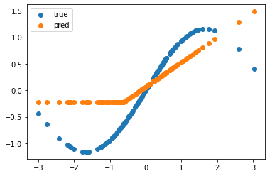
In this step, we plot the ground truth and predicted values. As shown in Figure 4, the model converges but could be more effective. It cannot fully capture the nonlinearity present in the data.

plt.scatter(xs, ys, label="true")
plt.scatter(xs, nonlinear_model(theta, xs), label="pred")
plt.legend()
plt.show()

---

🌲 Training with PyTrees

But why are we suddenly interested in linear and nonlinear models? Aren’t they a little too basic? It’s always best to revisit fundamentals and remember why we are learning a new technique. Otherwise, we will be left with the knowledge of many techniques but without wisdom on when to use them.

A linear model is a model that is based on a linear equation, meaning that the output is a linear combination of the inputs. While linear models are simple and easy to understand, they have some limitations when modeling nonlinear relationships. Nonlinear models, on the other hand, can overcome these limitations by allowing for more complex relationships between inputs and outputs.

However, these (nonlinear) models require more parameters to model nonlinear functions, which makes training them more complicated. One of the main issues with having more parameters is that we need to pass each through weights and biases and apply gradients on each individually. This is a lengthy process, and where PyTrees from JAX comes in.

A PyTree is a container that can hold leaf elements, which are non-container objects such as arrays and other PyTrees. This allows for nested structures, where the container types do not need to match. This means a PyTree can be a list, tuple, dictionary of leaf elements, or other PyTrees.

In the context of a neural network, a PyTree can be used to represent the weights and biases of the network. Instead of initializing a separate list for each weight and bias, a PyTree can be used as a container for all the weights and biases. This makes it easier to handle many parameters, as the PyTree can be easily iterated over and modified.

JAX provides built-in support for PyTrees through the jax.tree_utils module, which includes functions such as jax.tree_map and jax.tree_leaves to manipulate and traverse the PyTree easily. The most common functions are also available as jax.tree_*.

def init_mlp_params(layer_widths):
    """
    Function to initialize the parameters of a Multilayer Perceptron.

    Args:
        - layer_widths: The list of layer widths.
    
    Returns:
        Randomly initialized parameters of the model.
    """
    key = random.PRNGKey(42)
    
    # params of the MLP will be a pytree
    params = []
    for number_in, number_out in zip(layer_widths[:-1], layer_widths[1:]):
        key, subkey = random.split(key)
        params.append(
            dict(
                weights=random.normal(subkey, shape=(number_in, number_out)) * jnp.sqrt(2/number_in),
                biases=jnp.ones(shape=(number_out,))
            )
        )
    return params

The init_mlp_params function takes in a single argument, layer_widths, which is a list of each layer’s widths in an MLP model.

We then initialize an empty list called params, which will be used to store the parameters of the MLP as a PyTree.

The function then enters a for loop, iterating over the layer_widths list, using the zip function to pair the input and output number of neurons for each layer.

On each iteration of the loop, the function splits the key into two parts, the key and subkey, using the random.split function (read how JAX handles randomness in Part 2 of this series). Then it appends a dictionary to the params list, which contains two keys, weights and biases, each with its corresponding value.

The value of the weights key is a random normal distribution generated using the random.normal function, with shape (number_in, number_out), and it is scaled by jnp.sqrt(2/number_in), which is a common initialization technique to ensure that the variance of the input is preserved.

The value of the biases key is an array of ones with shape (number_out,).

Finally, the function returns the params list, which contains the initialized parameters of the MLP model as a PyTree.

# Initialize the parameters of the MLP
params = init_mlp_params([1, 128, 128, 1])

# Custom function to get shape
get_shape = lambda x:x.shape
shape_pytree = jax.tree_map(get_shape, params)

for idx, layer in enumerate(shape_pytree):
    print(f"Layer {idx}")
    print(layer)

We use the init_mlp_params defined previously to initialize the parameters of a multilayer perceptron (MLP) model with layer widths of [1, 128, 128, 1]. The returned parameters are stored in the variable parameters.

We define a lambda function get_shape, which takes a single argument x and returns its shape using the shape attribute.

The function jax.tree_map(get_shape, params) is called. This function applies the get_shape function to every leaf element in the params PyTree. The result is a new PyTree (shape_pytree), where the shape of the corresponding leaf element in params PyTree replaces each leaf element.

Finally, the code enters a for loop, iterating over the shape_pytree list. On each iteration, the loop prints the index of the current layer using the enumerate function and the shape of the current layer by accessing the current value in the shape_pytree list.

This code snippet can be used to check the shapes of the parameters of each layer of the MLP model. The output will show the number of neurons in the input and output layers of each layer of the MLP.

>>> Layer 0
>>> {'biases': (128,), 'weights': (1, 128)}
>>> Layer 1
>>> {'biases': (128,), 'weights': (128, 128)}
>>> Layer 2
>>> {'biases': (1,), 'weights': (128, 1)}

Now that we have our model initialized, we define the forward step.

def forward(params, x):
    """
    The forward propagation step.

    Args:
        - params: The parameters of the model.
        - x: The input to the model.
    
    Returns:
        Prediction from the model.
    """
    # Get the hidden layers and the last layer separately.
    *hidden, last = params

    # Iterate over the hidden layers and forward propagate the
    # input through the layers.
    for layer in hidden:
        x = jax.nn.relu(x @ layer["weights"] + layer["biases"])

    # Get the prediction
    pred = x @ last["weights"] + last["biases"]
    return pred

The forward function performs the forward propagation step of a neural network. The function uses two arguments, params and x.

The params argument is the model’s parameters, which is expected to be a PyTree containing the weights and biases for each network layer. The x argument is the input to the model.

The function starts by using an unpacking operator * to extract the hidden layers and the last layer from the params PyTree. It then enters a for loop, iterating over the hidden layers.

On each iteration, the function performs a matrix multiplication of the input x with the weights of the current layer, and adds the biases of the current layer. Then it applies the ReLU (Rectified Linear Unit) activation function to the result using the jax.nn.relu function.

This process is repeated for all hidden layers.

After the for loop, the function performs a matrix multiplication of the final output from the hidden layers with the weights of the last layer, and adds the biases of the last layer. This produces the final prediction from the model. Finally, the function returns the prediction.

def get_loss(params, x, y):
    """
    The loss function. We use the L2 distance as our loss function.

    Args:
        - params: Parameters of the model.
        - x: Input to the model.
        - y: The ground truth of the dataset.
    
    Returns:
        A scalar loss between the ground truth and the predicted value.
    """
    pred = forward(params, x)
    loss = jnp.mean((pred - y) ** 2)
    return loss

You might notice that the loss function get_loss is very similar to what we defined earlier. The only difference is with the params. Previously, params were tuples of parameters. Now the params are PyTrees consisting of the parameters of each layer of the MLP.

@jax.jit
def update_step(params, x, y, lr):
    """
    A single update step for our model. We use the simple stochastic
    gradient update as our optimizer.

    Args:
        - params: Parameters of the model.
        - x: Input to the model.
        - y: The ground truth of the dataset.
        - lr: Learning rate of the optimizer.
    
    Returns:
        - The current updated state of the model parameters.
        - The current loss
    """
    loss, gradients = jax.value_and_grad(get_loss)(params, x, y)
    sgd = lambda param, gradient: param - lr * gradient
    updated_params = jax.tree_map(
        sgd, params, gradients
    )
    return updated_params, loss

To this point, we have defined our model, the forward propagation step, and the loss function. The missing piece of training a neural network is the update_step.

The update_step function takes in four arguments: params, x, y, and lr. The params argument represents the model’s parameters, x represents the input to the model, y represents the ground truth of the dataset, and lr represents the learning rate of the optimizer.

The main motivation of the update_step function is to grab the gradient of the loss wrt the parameters and update the current parameters. The update should, in turn, optimize the loss function.

Here, the jax.value_and_grad function lets us compute the loss and the gradient. Now we define a lambda function sgd, which takes params and gradients and returns the updated params according to the stochastic gradient descent algorithm.

We use the jax.tree_map method to apply the sgd function to each leaf node in the params PyTree.

The reason behind using a PyTree should become clear now. We did not have to change our code much from that of linear and nonlinear model training. The only necessary change was to use the jax.tree_utils functions to include PyTree in the training procedure.

---

Train the MLP

We have all of our tools in hand. Let’s slay this monster now.

# Build the dataset
xs = random.normal(key, shape=(128, 1))

mu = 0.0
sigma = 0.1
noise = mu + sigma * random.normal(key, shape=(128, 1))

ys = jnp.sin(xs) + noise

We reuse the same code to build our nonlinear dataset with sinusoids and a pinch of noise.

epochs = 1000
for iter in range(epochs):
    params, loss = update_step(params, xs, ys, 1e-5)

    if iter % 100 == 0 and iter != 0:
        print(f"ITER {iter} | LOSS {loss:.4f}")

Using the same code to iterate through the dataset and update the model’s parameters.

>>> ITER 100 | LOSS 0.9694
>>> ITER 200 | LOSS 0.4728
>>> ITER 300 | LOSS 0.2778
>>> ITER 400 | LOSS 0.1969
>>> ITER 500 | LOSS 0.1600
>>> ITER 600 | LOSS 0.1404
>>> ITER 700 | LOSS 0.1279
>>> ITER 800 | LOSS 0.1185
>>> ITER 900 | LOSS 0.1107

And finally, plot our results to show the nonlinear model’s convergence rate. Figure 5 shows that our multilayer perceptron model has modeled on the dataset quite well.

plt.scatter(xs, ys, label="true")
plt.scatter(xs, forward(params, xs), label="pred")
plt.legend()
plt.show()

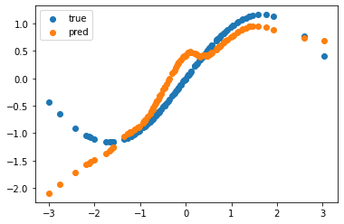
As shown in the plot, these powerful tools can expertly fit even the most nonlinear data with just a few parameters. Embrace the challenge and see what amazing results you can achieve with your own model and dataset. And don’t forget to share your stunning convergence plots on Twitter, tagging us for a chance to win a surprise!

---

---

Summary

So, we’ve covered a lot of ground in this blog post! We looked at how JAX can train linear and nonlinear regression models and even showed you how to use the PyTrees library to train a multilayer perceptron (MLP) model.

But that’s just the tip of the iceberg! We’re excited to inform you that this is just the first in a series of posts that will dive deeper into the world of JAX. We’ll cover more advanced topics and show you even more cool things you can do with this powerful library.

It’s no secret that JAX is becoming increasingly popular in machine learning, and the foundations we’ve covered here will be super useful in your future projects. So, watch out for our next posts, and let’s keep exploring the amazing world of JAX together!

---

Citation Information

A. R. Gosthipaty and R. Raha. “Learning JAX in 2023: Part 3 — A Step-by-Step Guide to Training Your First Machine Learning Model with JAX,” PyImageSearch, P. Chugh, S. Huot, K. Kidriavsteva, and A. Thanki, eds., 2023, https://pyimg.co/pidru

@incollection{ARG-RR_2023_Jax2023Pt3,
  author = {Aritra Roy Gosthipaty and Ritwik Raha},
  title = {Learning {JAX} in 2023: Part 3 — A Step-by-Step Guide to Training Your First Machine Learning Model with {JAX}},
  booktitle = {PyImageSearch},
  editor = {Puneet Chugh and Susan Huot and Kseniia Kidriavsteva and Abhishek Thanki},
  year = {2023},
  url = {https://pyimg.co/pidru},
}

---

---

To download the source code to this post (and be notified when future tutorials are published here on PyImageSearch), simply enter your email address in the form below!