Automatic Differentiation Part 2: Implementation Using Micrograd

---

Table of Contents

---

Automatic Differentiation Part 2: Implementation Using Micrograd

In this tutorial, you will learn how automatic differentiation works with the help of a Python package named micrograd.

This lesson is the last of a 2-part series on Autodiff 101 — Understanding Automatic Differentiation from Scratch:

1. Automatic Differentiation Part 1: Understanding the Math
2. Automatic Differentiation Part 2: Implementation Using Micrograd (today’s tutorial)

To learn how to implement automatic differentiation using Python, just keep reading.

---

Automatic Differentiation Part 2: Implementation Using Micrograd

---

Introduction

---

What Is a Neural Network?

A Neural Network is a mathematical abstraction of our brain (at least, that is how it all started). The system consists of many learnable knobs (weights and biases) and a simple operation (dot product). The Neural Network takes in inputs and uses an objective function that we need to optimize by turning the knobs. The best way to tune the knobs is to use the gradient of the objective function with respect to all the individual knobs as a signal.

It will take a long time if you sit down and try to calculate the gradient by hand. So, to bypass this process, we use the concept of automatic differentiation.

In the previous tutorial, we deeply studied the mathematics of automatic differentiation. This tutorial will apply the concepts and work our way into understanding an automatic differentiation Python package from scratch.

The package that we will talk about today is called micrograd. This is an open-source Python package created by Andrej Karpathy. We have studied the video lecture, where Andrej built the package from scratch. Here, we break down the video lecture into a blog where we add our thoughts to enrich the content.

---

Having Problems Configuring Your Development Environment?

All that said, are you:

• Short on time?
• Learning on your employer’s administratively locked system?
• Wanting to skip the hassle of fighting with the command line, package managers, and virtual environments?
• Ready to run the code right now on your Windows, macOS, or Linux system?

Then join PyImageSearch University today!

Gain access to Jupyter Notebooks for this tutorial and other PyImageSearch guides that are pre-configured to run on Google Colab’s ecosystem right in your web browser! No installation required.

And best of all, these Jupyter Notebooks will run on Windows, macOS, and Linux!

---

About micrograd

micrograd is a Python package built to understand how the reverse accumulation (backpropagation) process works in a modern deep learning package like PyTorch or Jax. It is a simple automatic differentiation package that works with scalars only.

---

Imports and Setup

import math
import random
from typing import List, Tuple, Union
from matplotlib import pyplot as plt

---

The Value Class

We start things off by defining the Value class. To work on tracing and backpropagation later, it becomes essential to wrap raw scalar values into the Value class.

When wrapped inside the Value class, the scalar value is considered a Node of a Graph. When we use Values and build an equation, the equation is considered a Directed Acyclic Graph (DAG). With the help of calculus and graph traversal, we compute the gradients of the nodes automatically (autodiff) and backpropagate through them.

The Value class has the following attributes:

• data: The raw float data that needs to be wrapped inside the Value class.
• grad: This will hold the global derivative of the node. The global derivative is the partial derivative of the root node (final node) with respect to the current node.
• _backward: This is a private method that computes the global derivative of the children of the current node.
• _prev: The children of the current node.

class Value(object):
    """
    We need to wrap the raw data into a class that will store the
    metadata to help in automatic differentiation.

    Attributes:
        data (float): The data for the Value node.
        _children (Tuple): The children of the current node.
    """

    def __init__(self, data: float, _children: Tuple = ()):
        # The raw data for the Value node.
        self.data = data

        # The partial gradient of the last node with respect to this
        # node. This is also termed as the global gradient.
        # Gradient 0.0 means that there is no effect of the change
        # of the last node with respect to this node. On
        # initialization it is assumed that all the variables have no
        # effect on the entire architecture.
        self.grad = 0.0

        # The function that derives the gradient of the children nodes
        # of the current node. It is easier this way, because each node
        # is built from children nodes and an operation. Upon back-propagation
        # the current node can easily fill in the gradients of the children.
        # Note: The global gradient is the multiplication of the local gradient
        # and the flowing gradient from the parent.
        self._backward = lambda: None

        # Define the children of this node.
        self._prev = set(_children)

    def __repr__(self):
        # This is the string representation of the Value node.
        return f"Value(data={self.data}, grad={self.grad})"

# Build a Value node
raw_data = 5.0
print(f"Raw Data(data={raw_data}, type={type(raw_data)}")
value_node = Value(data=raw_data)

# Calling the `__repr__` function here
print(value_node)

>>> Raw Data(data=5.0, type=<class 'float'>
>>> Value(data=5.0, grad=0.0)

---

Addition

Now that we have built our Value class, we need to define the primitive operations and their _backward functions. This will help trace each node’s operations and back-propagate the gradients through the DAG expression.

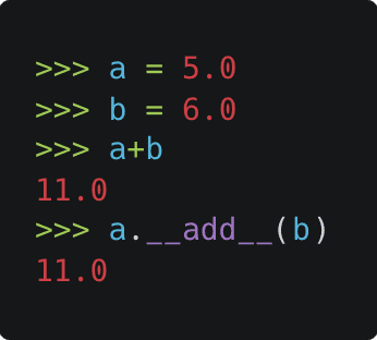
In this section, we deal with the addition operation. This will help in two values being added together. Python classes have a special method __add__ called when we use the + operator, as shown in Figure 1.

Here we create the custom_addition function that is later assigned to the __add__ method of the Value class. This is done for us to focus on the addition method and discard everything that is not important to the addition operation.

The addition operation is as simple as it gets:

1. The self and the other nodes as an argument to the call. We then take their data and apply addition.
2. The result is then wrapped inside the Value class.
3. The out node is initialized, where we mention that self and other are its children.

---

Compute Gradient

We will have this section for every primitive operation that we define. For example, to compute the global gradient of the children nodes, we need to define the local gradient of the addition operation.

Let us consider a node that is built by adding two children nodes and . Then, the partial derivatives of are derived in Figure 2.

Now think of backpropagation. The partial derivative of the loss (objective) function is already deduced for . This means we have . This gradient needs to flow to the child nodes and , respectively.

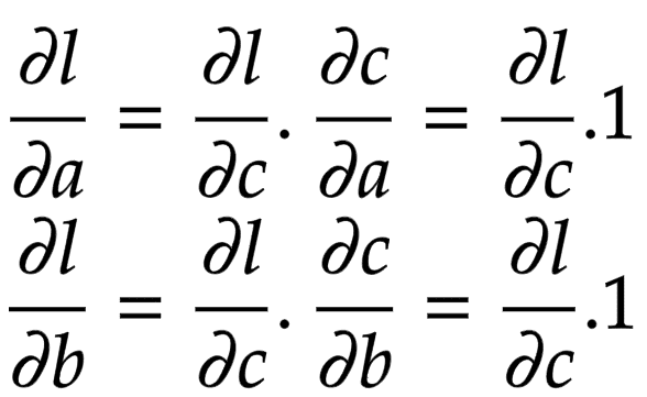
Applying the chain rule, we get the global gradient for and , as shown in Figure 3.

The addition operation acts like a router to the gradients flowing in. It routes the gradients to all the children.

➤ Note: In the _backward functions that we define, we accumulate the gradients of the children with the += operation. This is done to bypass a unique case. Suppose we have . Here we know that the expression can be simplified to , but our _backward for __add__ does not know how to do this. The __backward__ in __add__ treats one as self and the other as other. If the gradients are not accumulated, we will see a discrepancy with the gradients.

def custom_addition(self, other: Union["Value", float]) -> "Value":
    """
    The addition operation for the Value class.
    Args:
        other (Union["Value", float]): The other value to add to this one.
    Usage:
        >>> x = Value(2)
        >>> y = Value(3)
        >>> z = x + y
        >>> z.data
        5
    """
    # If the other value is not a Value, then we need to wrap it.
    other = other if isinstance(other, Value) else Value(other)

    # Create a new Value node that will be the output of the addition.
    out = Value(data=self.data + other.data, _children=(self, other))

    def _backward():
        # Local gradient:
        # x = a + b
        # dx/da = 1
        # dx/db = 1
        # Global gradient with chain rule:
        # dy/da = dy/dx . dx/da = dy/dx . 1
        # dy/db = dy/dx . dx/db = dy/dx . 1
        self.grad += out.grad * 1.0
        other.grad += out.grad * 1.0

    # Set the backward function on the output node.
    out._backward = _backward
    return out

def custom_reverse_addition(self, other):
    """
    Reverse addition operation for the Value class.
    Args:
        other (float): The other value to add to this one.
    Usage:
        >>> x = Value(2)
        >>> y = Value(3)
        >>> z = y + x
        >>> z.data
        5
    """
    # This is the same as adding. We can reuse the __add__ method.
    return self + other


Value.__add__ = custom_addition
Value.__radd__ = custom_reverse_addition

# Build a and b
a = Value(data=5.0)
b = Value(data=6.0)

# Print the addition
print(f"{a} + {b} => {a+b}")

>>> Value(data=5.0, grad=0.0) + Value(data=6.0, grad=0.0) => Value(data=11.0, grad=0.0)

# Add a and b
c = a + b

# Assign a global gradient to c
c.grad = 11.0
print(f"c => {c}")

# Now apply `_backward` to c
c._backward()
print(f"a => {a}")
print(f"b => {b}")

>>> c => Value(data=11.0, grad=11.0)
>>> a => Value(data=5.0, grad=11.0)
>>> b => Value(data=6.0, grad=11.0)

➤ Note: The global gradient of is routed to and .

---

Multiplication

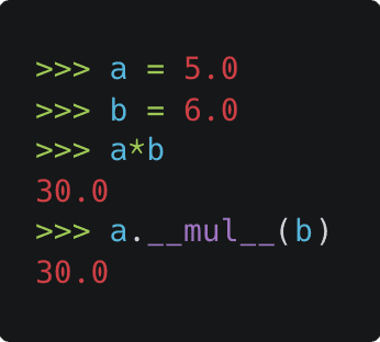
In this section, we deal with the multiplication operation. Python classes have a special method __mul__ called when we use the * operator, as shown in Figure 4.

We get the self and the other nodes as an argument to the call. We then take their data and apply multiplication. The result is then wrapped inside the Value class. Finally, the out node is initialized, where we mention that self and other are its children.

---

Compute Gradient

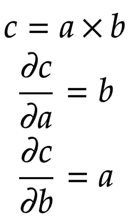
Let us consider a node that is built by multiplying two children nodes and . Then, the partial derivatives of are shown in Figure 5.

Now think of backpropagation. The partial derivative of the loss (objective) function is already deduced for . This means we have . This gradient needs to flow to the children nodes and , respectively.

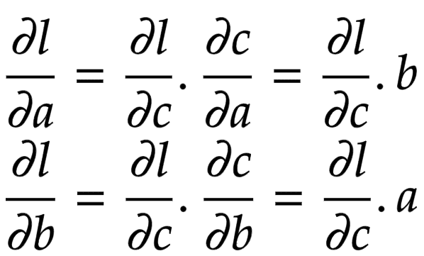
Applying the chain rule, we get the global gradient for and , as shown in Figure 6.

def custom_multiplication(self, other: Union["Value", float]) -> "Value":
    """
    The multiplication operation for the Value class.
    Args:
        other (float): The other value to multiply to this one.
    Usage:
        >>> x = Value(2)
        >>> y = Value(3)
        >>> z = x * y
        >>> z.data
        6
    """
    # If the other value is not a Value, then we need to wrap it.
    other = other if isinstance(other, Value) else Value(other)

    # Create a new Value node that will be the output of
    # the multiplication.
    out = Value(data=self.data * other.data, _children=(self, other))

    def _backward():
        # Local gradient:
        # x = a * b
        # dx/da = b
        # dx/db = a
        # Global gradient with chain rule:
        # dy/da = dy/dx . dx/da = dy/dx . b
        # dy/db = dy/dx . dx/db = dy/dx . a
        self.grad += out.grad * other.data
        other.grad += out.grad * self.data

    # Set the backward function on the output node.
    out._backward = _backward
    return out

def custom_reverse_multiplication(self, other):
    """
    Reverse multiplication operation for the Value class.
    Args:
        other (float): The other value to multiply to this one.
    Usage:
        >>> x = Value(2)
        >>> y = Value(3)
        >>> z = y * x
        >>> z.data
        6
    """
    # This is the same as multiplying. We can reuse the __mul__ method.
    return self * other


Value.__mul__ = custom_multiplication
Value.__rmul__ = custom_reverse_multiplication

# Build a and b
a = Value(data=5.0)
b = Value(data=6.0)

# Print the multiplication
print(f"{a} * {b} => {a*b}")

>>> Value(data=5.0, grad=0.0) * Value(data=6.0, grad=0.0) => Value(data=30.0, grad=0.0)

# Multiply a and b
c = a * b

# Assign a global gradient to c
c.grad = 11.0
print(f"c => {c}")

# Now apply `_backward` to c
c._backward()
print(f"a => {a}")
print(f"b => {b}")

>>> c => Value(data=30.0, grad=11.0)
>>> a => Value(data=5.0, grad=66.0)
>>> b => Value(data=6.0, grad=55.0)

---

Power

In this section, we deal with the power operation. Python classes have a special method __pow__ that is called when we use the ** operator, as shown in Figure 7.

After obtaining the self and the other nodes as an argument to the call, we take their data and apply the power operation.

---

Compute Gradient

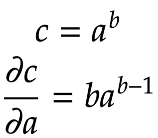
Let us consider a node that is built by multiplying two children nodes and . Then, the partial derivatives of are derived in Figure 8.

Now think of backpropagation. The partial derivative of the loss (objective) function is already deduced for . This means we have . This gradient needs to flow to the child node .

Applying the chain rule, we get the global gradient for and , as shown in Figure 9.

def custom_power(self, other):
    """
    The power operation for the Value class.
    Args:
        other (float): The other value to raise this one to.
    Usage:
        >>> x = Value(2)
        >>> z = x ** 2.0
        >>> z.data
        4
    """
    assert isinstance(
        other, (int, float)
    ), "only supporting int/float powers for now"

    # Create a new Value node that will be the output of the power.
    out = Value(data=self.data ** other, _children=(self,))

    def _backward():
        # Local gradient:
        # x = a ** b
        # dx/da = b * a ** (b - 1)
        # Global gradient:
        # dy/da = dy/dx . dx/da = dy/dx . b * a ** (b - 1)
        self.grad += out.grad * (other * self.data ** (other - 1))

    # Set the backward function on the output node.
    out._backward = _backward
    return out


Value.__pow__ = custom_power

# Build a
a = Value(data=5.0)
# For power operation we will use
# the raw data and not wrap it into
# a node. This is done for simplicity.
b = 2.0

# Print the power operation
print(f"{a} ** {b} => {a**b}")

>>> Value(data=5.0, grad=0.0) ** 2.0 => Value(data=25.0, grad=0.0)

# Raise a to the power of b
c = a ** b

# Assign a global gradient to c
c.grad = 11.0
print(f"c => {c}")

# Now apply `_backward` to c
c._backward()
print(f"a => {a}")
print(f"b => {b}")

>>> c => Value(data=25.0, grad=11.0)
>>> a => Value(data=5.0, grad=110.0)
>>> b => 2.0

---

Negation

For the negation operation, we will be using the __mul__ operation defined above. In addition, Python classes have a special method __neg__ called when we use the unary - operator, as shown in Figure 10.

This means the _backward of negation will be taken care of, and we would not have to define it explicitly.

def custom_negation(self):
    """
    Negation operation for the Value class.
    Usage:
        >>> x = Value(2)
        >>> z = -x
        >>> z.data
        -2
    """
    # This is the same as multiplying by -1. We can reuse the
    # __mul__ method.
    return self * -1

Value.__neg__ = custom_negation

# Build `a`
a = Value(data=5.0)

# Print the negation
print(f"Negation of {a} => {(-a)}")

>>> Negation of Value(data=5.0, grad=0.0) => Value(data=-5.0, grad=0.0)

# Negate a
c = -a

# Assign a global gradient to c
c.grad = 11.0
print(f"c => {c}")

# Now apply `_backward` to c
c._backward()
print(f"a => {a}")

>>> c => Value(data=-5.0, grad=11.0)
>>> a => Value(data=5.0, grad=-11.0)

---

Subtraction

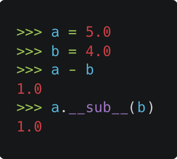
The subtraction operation can be handled with __add__ and __neg__. In addition, Python classes have a special method __sub__ called when we use the - operator, as shown in Figure 11.

This will help us delegate the _backward subtraction operation to the addition and negation operations.

def custom_subtraction(self, other):
    """
    Subtraction operation for the Value class.
    Args:
        other (float): The other value to subtract to this one.
    Usage:
        >>> x = Value(2)
        >>> y = Value(3)
        >>> z = x - y
        >>> z.data
        -1
    """
    # This is the same as adding the negative of the other value.
    # We can reuse the __add__ and the __neg__ methods.
    return self + (-other)

def custom_reverse_subtraction(self, other):
    """
    Reverse subtraction operation for the Value class.
    Args:
        other (float): The other value to subtract to this one.
    Usage:
        >>> x = Value(2)
        >>> y = Value(3)
        >>> z = y - x
        >>> z.data
        1
    """
    # This is the same as subtracting. We can reuse the __sub__ method.
    return other + (-self)


Value.__sub__ = custom_subtraction
Value.__rsub__ = custom_reverse_subtraction

# Build a and b
a = Value(data=5.0)
b = Value(data=4.0)

# Print the negation
print(f"{a} - {b} => {(a-b)}")

>>> Value(data=5.0, grad=0.0) - Value(data=4.0, grad=0.0) => Value(data=1.0, grad=0.0)

# Subtract b from a
c = a - b

# Assign a global gradient to c
c.grad = 11.0
print(f"c => {c}")

# Now apply `_backward` to c
c._backward()
print(f"a => {a}")
print(f"b => {b}")

>>> c => Value(data=1.0, grad=11.0)
>>> a => Value(data=5.0, grad=11.0)
>>> b => Value(data=4.0, grad=0.0)

➤ Note: The gradients did not flow as they were supposed to on paper. Why? Can you figure out the answer to this?

➤ Hint: The subtraction operation consists of more than one primitive operation: negation and addition.

We will discuss this later in the tutorial.

---

Division

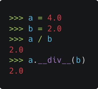
The division operation can be handled with __mul__ and __pow__. In addition, Python classes have a special method __div__ called when we use the / operator, as shown in Figure 12.

This will help us delegate the _backward division operation to the power operation.

def custom_division(self, other):
    """
    Division operation for the Value class.
    Args:
        other (float): The other value to divide to this one.
    Usage:
        >>> x = Value(10)
        >>> y = Value(5)
        >>> z = x / y
        >>> z.data
        2
    """
    # Use the __pow__ method to implement division.
    return self * other ** -1

def custom_reverse_division(self, other):
    """
    Reverse division operation for the Value class.
    Args:
        other (float): The other value to divide to this one.
    Usage:
        >>> x = Value(10)
        >>> y = Value(5)
        >>> z = y / x
        >>> z.data
        0.5
    """
    # Use the __pow__ method to implement division.
    return other * self ** -1


Value.__truediv__ = custom_division
Value.__rtruediv__ = custom_reverse_division

# Build a and b
a = Value(data=6.0)
b = Value(data=3.0)

# Print the negation
print(f"{a} / {b} => {(a/b)}")

>>> Value(data=6.0, grad=0.0) / Value(data=3.0, grad=0.0) => Value(data=2.0, grad=0.0)

# Divide a with b
c = a / b

# Assign a global gradient to c
c.grad = 11.0
print(f"c => {c}")

# Now apply `_backward` to c
c._backward()
print(f"a => {a}")
print(f"b => {b}")

>>> c => Value(data=2.0, grad=11.0)
>>> a => Value(data=6.0, grad=3.6666666666666665)
>>> b => Value(data=3.0, grad=0.0)

➤ With division, we see the same problem with gradient flow as we had seen with subtraction. Have you figured out the problem yet? 👀

---

Rectified Linear Unit

In this section, we introduce nonlinearity. ReLU is not a primitive function; we would need to build the function and also the _backward function for it.

def relu(self):
    """
    The ReLU activation function.
    Usage:
        >>> x = Value(-2)
        >>> y = x.relu()
        >>> y.data
        0
    """
    out = Value(data=0 if self.data < 0 else self.data, _children=(self,))

    def _backward():
        # Local gradient:
        # x = relu(a)
        # dx/da = 0 if a < 0 else 1
        # Global gradient:
        # dy/da = dy/dx . dx/da = dy/dx . (0 if a < 0 else 1)
        self.grad += out.grad * (out.data > 0)

    # Set the backward function on the output node.
    out._backward = _backward
    return out


Value.relu = relu

# Build a
a = Value(data=6.0)

# Print a and the negation
print(f"ReLU ({a}) => {(a.relu())}")
print(f"ReLU (-{a}) => {((-a).relu())}")

>>> ReLU (Value(data=6.0, grad=0.0)) => Value(data=6.0, grad=0.0)
>>> ReLU (-Value(data=6.0, grad=0.0)) => Value(data=0, grad=0.0)

# Build a and b
a = Value(3.0)
b = Value(-3.0)

# Apply relu on both the nodes
relu_a = a.relu()
relu_b = b.relu()

# Assign a global gradients
relu_a.grad = 11.0
relu_b.grad = 11.0

# Now apply `_backward`
relu_a._backward()
print(f"a => {a}")
relu_b._backward()
print(f"b => {b}")

>>> a => Value(data=3.0, grad=11.0)
>>> b => Value(data=-3.0, grad=0.0)

---

The Global Backward

Until now, we have devised primitive and non-primitive (ReLU) functions with their individual _backward methods. Each primitive can back-prop the flowing gradients to its children only.

We now have to devise a method to iterate over all such primitive methods in a DAG (built equation) and back-propagate the gradient over the entire expression.

To make that happen, the Value call needs a global backward method. We apply the backward function on the last (final) node of the DAG. The function performs the following operations:

• Sorts the DAG in a topological order
• Sets the grad of the last node as 1.0
• Iterates over the topologically sorted graph and applies the _backward method of each primitive.

def backward(self):
    """
    The backward pass of the backward propagation algorithm.
    Usage:
        >>> x = Value(2)
        >>> y = Value(3)
        >>> z = x * y
        >>> z.backward()
        >>> x.grad
        3
        >>> y.grad
        2
    """
    # Build an empty list which will hold the
    # topologically sorted graph
    topo = []

    # Build a set of all the visited nodes
    visited = set()

    # A closure to help build the topologically sorted graph
    def build_topo(node: "Value"):
        if node not in visited:
            # If node is not visited add the node to the
            # visited set.
            visited.add(node)

            # Iterate over the children of the node that
            # is being visited
            for child in node._prev:
                # Apply recursion to build the topologically sorted
                # graph of the children
                build_topo(child)
            
            # Only append node to the topologically sorted list
            # if all its children are visited.
            topo.append(node)

    # Call the `build_topo` method on self
    build_topo(self)

    # Go one node at a time and apply the chain rule
    # to get its gradient
    self.grad = 1.0
    for node in reversed(topo):
        node._backward()

Value.backward = backward

# Now create an expression that uses a lot of
# primitive operations
a = Value(2.0)
b = Value(3.0)
c = a+b
d = 4.0
e = c**d
f = Value(6.0)
g = e/f


print(“BEFORE backward”)
for element in [a, b, c, d, e, f, g]:
    print(element)

# Backward on the final node will backprop
# the gradients through the entire DAG
g.backward()


print(“AFTER backward”)
for element in [a, b, c, d, e, f, g]:
    print(element)

>>> BEFORE backward
>>> Value(data=2.0, grad=0.0)
>>> Value(data=3.0, grad=0.0)
>>> Value(data=5.0, grad=0.0)
>>> 4.0
>>> Value(data=625.0, grad=0.0)
>>> Value(data=6.0, grad=0.0)
>>> Value(data=104.16666666666666, grad=0.0)

>>> AFTER backward
>>> Value(data=2.0, grad=83.33333333333333)
>>> Value(data=3.0, grad=83.33333333333333)
>>> Value(data=5.0, grad=83.33333333333333)
>>> 4.0
>>> Value(data=625.0, grad=0.16666666666666666)
>>> Value(data=6.0, grad=-17.36111111111111)
>>> Value(data=104.16666666666666, grad=1.0)

Remember the problem we had with __sub__ and __div__? The gradients did not backpropagate according to the rules of calculus. There is nothing wrong with implementing the _backward function.

However, the two operations (__sub__ and __div__) are built with more than one primitive operation (__neg__ and __add__ for __sub__; __mul__ and __pow__ for __div__).

This creates an intermediate node that prohibits the gradients from flowing to the children properly (remember, _backward is not supposed to backpropagate the gradients through the entire DAG).

# Solve the problem with subtraction
a = Value(data=6.0)
b = Value(data=3.0)

c = a - b
c.backward()
print(f"c => {c}")
print(f"a => {a}")
print(f"b => {b}")

c => Value(data=3.0, grad=1.0)
a => Value(data=6.0, grad=1.0)
b => Value(data=3.0, grad=-1.0)

# Solve the problem with division
a = Value(data=6.0)
b = Value(data=3.0)

c = a / b
c.backward()
print(f"c => {c}")
print(f"a => {a}")
print(f"b => {b}")

>>> c => Value(data=2.0, grad=1.0)
>>> a => Value(data=6.0, grad=0.3333333333333333)
>>> b => Value(data=3.0, grad=-0.6666666666666666)

---

Build a Multilayer Perceptron with micrograd

What good does it do if we just build the Value class and not build a Neural Network with it?

In this section, we build a very simple Neural Network (a Multilayer Perceptron) and use it to model a simple dataset.

---

Module

This is the parent class. The Module class has two methods:

• zero_grad: This is used to zero out all the gradients of the parameters.
• parameters: This function is built to be overwritten. This would eventually get us the parameters of the neurons, layers, and the mlp.

class Module(object):
    """
    The parent class for all neural network modules.
    """

    def zero_grad(self):
        # Zero out the gradients of all parameters.
        for p in self.parameters():
            p.grad = 0

    def parameters(self):
        # Initialize a parameters function that all the children will
        # override and return a list of parameters.
        return []

---

Neuron

This serves as the unit of our Neural Network upon which the entire architecture is built. It has a list of weights and a bias. The function of a Neuron is shown in Figure 13.

class Neuron(Module):
    """
    A single neuron.
    Parameters:
        number_inputs (int): number of inputs
        is_nonlinear (bool): whether to apply ReLU nonlinearity
        name (int): the index of neuron
    """

    def __init__(self, number_inputs: int, name, is_nonlinear: bool = True):
        # Create weights for the neuron. The weights are initialized
        # from a random uniform distribution.
        self.weights = [Value(data=random.uniform(-1, 1)) for _ in range(number_inputs)]

        # Create bias for the neuron.
        self.bias = Value(data=0.0)
        self.is_nonlinear = is_nonlinear

        self.name = name

    def __call__(self, x: List["Value"]) -> "Value":
        # Compute the dot product of the input and the weights. Add the
        # bias to the dot product.
        act = sum(
            ((wi * xi) for wi, xi in zip(self.weights, x)),
            self.bias
        )

        # If activation is mentioned, apply ReLU to it.
        return act.relu() if self.is_nonlinear else act

    def parameters(self):
        # Get the parameters of the neuron. The parameters of a neuron
        # is its weights and bias.
        return self.weights + [self.bias]

    def __repr__(self):
        # Print a better representation of the neuron.
        return f"Neuron {self.name}(Number={len(self.weights)}, Non-Linearity={'ReLU' if self.is_nonlinear else 'None'})"

x = [2.0, 3.0]
neuron = Neuron(number_inputs=2, name=1)
print(neuron)
out = neuron(x)
print(f"Output => {out}")

>>> Neuron 1(Number=2, Non-Linearity=ReLU)
>>> Output => Value(data=2.3063230206881347, grad=0.0)

---

Layer

A layer is built of a number of Neurons.

class Layer(Module):
    """
    A layer of neurons.
    Parameters:
        number_inputs (int): number of inputs
        number_outputs (int): number of outputs
        name (int): index of the layer
    """

    def __init__(self, number_inputs: int, number_outputs: int, name: int, **kwargs):
        # A layer is a list of neurons.
        self.neurons = [
            Neuron(number_inputs=number_inputs, name=idx, **kwargs) for idx in range(number_outputs)
        ]
        self.name = name
        self.number_outputs = number_outputs

    def __call__(self, x: List["Value"]) -> Union[List["Value"], "Value"]:
        # Iterate over all the neurons and compute the output of each.
        out = [n(x) for n in self.neurons]
        return out if self.number_outputs != 1 else out[0]

    def parameters(self):
        # The parameters of a layer is the parameters of all the neurons.
        return [p for n in self.neurons for p in n.parameters()]

    def __repr__(self):
        # Print a better representation of the layer.
        layer_str = "\n".join(f'    - {str(n)}' for n in self.neurons)
        return f"Layer {self.name} \n{layer_str}\n"

x = [2.0, 3.0]
layer = Layer(number_inputs=2, number_outputs=3, name=1)
print(layer)
out = layer(x)
print(f"Output => {out}")

>>> Layer 1 
>>>     - Neuron 0(Number=2, Non-Linearity=ReLU)
>>>     - Neuron 1(Number=2, Non-Linearity=ReLU)
>>>     - Neuron 2(Number=2, Non-Linearity=ReLU)

>>> Output => [Value(data=0, grad=0.0), Value(data=1.1705131190055296, grad=0.0), Value(data=3.0608608028649344, grad=0.0)]

x = [2.0, 3.0]
layer = Layer(number_inputs=2, number_outputs=1, name=1)
print(layer)
out = layer(x)
print(f"Output => {out}")

>>> Layer 1 
>>>     - Neuron 0(Number=2, Non-Linearity=ReLU)

>>> Output => Value(data=2.3123867684232247, grad=0.0)

---

Multilayer Perceptron

A Multilayer Perceptron (MLP) is built of a number of Layers.

class MLP(Module):
    """
    The Multi-Layer Perceptron (MLP) class.
    Parameters:
        number_inputs (int): number of inputs.
        list_number_outputs (List[int]): number of outputs in each layer.
    """

    def __init__(self, number_inputs: int, list_number_outputs: List[int]):
        # Get the number of inputs and all the number of outputs in
        # a single list.
        total_size = [number_inputs] + list_number_outputs

        # Build layers by connecting each layer to the previous one.
        self.layers = [
            # Do not use non linearity in the last layer.
            Layer(
                number_inputs=total_size[i],
                number_outputs=total_size[i + 1],
                name=i,
                is_nonlinear=i != len(list_number_outputs) - 1
            )
            for i in range(len(list_number_outputs))
        ]

    def __call__(self, x: List["Value"]) -> List["Value"]:
        # Iterate over the layers and compute the output of
        # each sequentially.
        for layer in self.layers:
            x = layer(x)
        return x

    def parameters(self):
        # Get the parameters of the MLP
        return [p for layer in self.layers for p in layer.parameters()]

    def __repr__(self):
        # Print a better representation of the MLP.
        mlp_str = "\n".join(f'  - {str(layer)}' for layer in self.layers)
        return f"MLP of \n{mlp_str}"

x = [2.0, 3.0]
mlp = MLP(number_inputs=2, list_number_outputs=[3, 3, 1])
print(mlp)
out = mlp(x)
print(f"Output => {out}")

>>> MLP of 
>>>   - Layer 0 
>>>     - Neuron 0(Number=2, Non-Linearity=ReLU)
>>>     - Neuron 1(Number=2, Non-Linearity=ReLU)
>>>     - Neuron 2(Number=2, Non-Linearity=ReLU)

>>>   - Layer 1 
>>>     - Neuron 0(Number=3, Non-Linearity=ReLU)
>>>     - Neuron 1(Number=3, Non-Linearity=ReLU)
>>>     - Neuron 2(Number=3, Non-Linearity=ReLU)

>>>   - Layer 2 
>>>     - Neuron 0(Number=3, Non-Linearity=None)

>>> Output => Value(data=-0.3211612402687316, grad=0.0)

---

Train the MLP

In this section, we will create a small dataset and try to understand how to model the dataset with our MLP.

# Build a dataset
xs = [
    [0.5, 0.5, 0.70],
    [0.4, -0.1, 0.5],
    [-0.2, -0.75, 1.0],
]
ys = [0.0, 1.0, 0.0]

# Build an MLP
mlp = MLP(number_inputs=3, list_number_outputs=[3, 3, 1])

In the following code snippet, we define three functions:

• forward: The forward function takes the mlp and the inputs. The inputs are forwarded through the mlp, and we obtain the predictions from the mlp.
• compute_loss: We have ground truth and predictions. This function computes the loss between the two. We will optimize our mlp to make the loss go to zero.
• update_mlp: In this function, we update the parameters (weights and biases) of our mlp with the gradient information.

def forward(mlp: "MLP", xs: List[List[float]]) -> List["Value"]:
    # Get the predictions upon forwarding the input data through
    # the mlp
    ypred = [mlp(x) for x in xs]
    return ypred

def compute_loss(ys: List[int], ypred: List["Value"]) -> "Value":
    # Obtain the L2 distance of the prediction and ground truths
    loss = sum(
        [(ygt - yout)**2 for ygt, yout in zip(ys, ypred)]
    )
    return loss

def update_mlp(mlp: "MLP"):
    # Iterate over all the layers of the MLP
    for layer in mlp.layers:
        # Iterate over all the neurons of each layer
        for neuron in layer.neurons:
            # Iterate over all the weights of each neuron
            for weight in neuron.weights:
                # Update the data of the weight with the 
                # gradient information.
                weight.data -= (1e-2 * weight.grad)
            # Update the data of the bias with the 
            # gradient information.
            neuron.bias.data -= (1e-2 * neuron.bias.grad)

# Define the epochs for which we want to run the training process.
epochs = 50

# Define a loss list to help log the loss.
loss_list = []

# Iterate each epoch and train the model.
for idx in range(epochs):
    # Step 1: Forward the inputs to the mlp and get the predictions
    ypred = forward(mlp, xs)
    # Step 2: Compute Loss between the predictions and the ground truths
    loss = compute_loss(ys, ypred)
    # Step 3: Ground the gradients. These accumulate which is not desired.
    mlp.zero_grad()
    # Step 4: Backpropagate the gradients through the entire architecture
    loss.backward()
    # Step 5: Update the mlp
    update_mlp(mlp)
    # Step 6: Log the loss
    loss_list.append(loss.data)
    print(f"Epoch {idx}: Loss {loss.data: 0.2f}")

Epoch 0: Loss  0.95
Epoch 1: Loss  0.89
Epoch 2: Loss  0.81
Epoch 3: Loss  0.74
Epoch 4: Loss  0.68
Epoch 5: Loss  0.63
Epoch 6: Loss  0.59
.
.
Epoch 47: Loss  0.24
Epoch 48: Loss  0.23
Epoch 49: Loss  0.22

# Plot the loss
plt.plot(loss_list)
plt.grid()
plt.ylabel("Loss")
plt.xlabel("Epoch")
plt.show()

The loss plot is shown in Figure 14.

# Inference
pred = mlp(xs[0])
ygt = ys[0]

print(f"Prediction => {pred.data: 0.2f}")
print(f"Ground Truth => {ygt: 0.2f}")

>>> Prediction =>  0.14
>>> Ground Truth =>  0.00

---

---

Summary

Our main objective with this blog post was to look under the hood of the autodiff process. With the help of Andrej’s micrograd repository, we now know how to shape a very minimal but working autodiff package.

We hope that the core concepts of autodiff, backpropagation, and basic neural network training are clear to you now.

Let us know how you liked this tutorial.

Twitter: @PyImageSearch

---

Citation Information

A. R. Gosthipaty and R. Raha. “Automatic Differentiation Part 2: Implementation Using Micrograd,” PyImageSearch, P. Chugh, S. Huot, K. Kidriavsteva, and A. Thanki, 2022, https://pyimg.co/ra6ow

@incollection{ARG-RR_2022_autodiff2,
  author = {Aritra Roy Gosthipaty and Ritwik Raha},
  title = {Automatic Differentiation Part 2: Implementation Using Micrograd},
  booktitle = {PyImageSearch},
  editor = {Puneet Chugh and Susan Huot and Kseniia Kidriavsteva and Abhishek Thanki},
  year = {2022},
  note = {https://pyimg.co/ra6ow},
}

---

---

To download the source code to this post (and be notified when future tutorials are published here on PyImageSearch), simply enter your email address in the form below!