A Deep Dive into Transformers with TensorFlow and Keras: Part 3

---

Table of Contents

---

A Deep Dive into Transformers with TensorFlow and Keras: Part 3

In this tutorial, you will learn how to code a transformer architecture from scratch in TensorFlow and Keras.

This lesson is the last in a 3-part series on NLP 104:

1. A Deep Dive into Transformers with TensorFlow and Keras: Part 1
2. A Deep Dive into Transformers with TensorFlow and Keras: Part 2
3. A Deep Dive into Transformers with TensorFlow and Keras: Part 3 (today’s tutorial)

To learn how to build a Transformer architecture using TensorFlow and Keras, just keep reading.

---

A Deep Dive into Transformers with TensorFlow and Keras: Part 3

We are at the third and final part of the series on Transformers. In Part 1, we learned about the evolution of attention from a simple feed-forward network to the current multi-head self-attention. Next, in Part 2, we focused on the connecting wires, the various components besides attention, that hold the architecture together.

This part of the tutorial will focus primarily on building a transformer from scratch using TensorFlow and Keras and applying it to the task of Neural Machine Translation. For the code, we have been heavily inspired by the official TensorFlow blog post on Transformers.

As discussed, we will understand how to build each component and finally stitch it together to train our own Transformer model.

---

Introduction

In the previous tutorials, we covered every component and module required for building the Transformer architecture. In this blog post, we will revisit those components and see how we can build those modules using TensorFlow and Keras.

We will then lay out the training pipeline and the inference script required to train and test the entire Transformer Architecture.

Here is a Hugging Face Spaces demo that shows the model trained on just 25 epochs. The purpose of this space is not to challenge Google Translate but to show how easy it is to train your model with our code and put it in production.

---

Configuring Your Development Environment

To follow this guide, you need to have tensorflow and tensorflow-text installed on your system.

Luckily, TensorFlow is pip-installable:

$ pip install tensorflow==2.8.0
$ pip install tensorflow-text==2.8.0

---

Having Problems Configuring Your Development Environment?

All that said, are you:

• Short on time?
• Learning on your employer’s administratively locked system?
• Wanting to skip the hassle of fighting with the command line, package managers, and virtual environments?
• Ready to run the code right now on your Windows, macOS, or Linux system?

Then join PyImageSearch University today!

Gain access to Jupyter Notebooks for this tutorial and other PyImageSearch guides that are pre-configured to run on Google Colab’s ecosystem right in your web browser! No installation required.

And best of all, these Jupyter Notebooks will run on Windows, macOS, and Linux!

---

Project Structure

We first need to review our project directory structure.

Start by accessing the “Downloads” section of this tutorial to retrieve the source code and example images.

From there, take a look at the directory structure:

$ tree .
.
├── inference.py
├── pyimagesearch
│   ├── attention.py
│   ├── config.py
│   ├── dataset.py
│   ├── decoder.py
│   ├── encoder.py
│   ├── feed_forward.py
│   ├── __init__.py
│   ├── loss_accuracy.py
│   ├── positional_encoding.py
│   ├── rate_schedule.py
│   ├── transformer.py
│   └── translate.py
└── train.py

1 directory, 14 files

In the pyimagesearch directory, we have the following:

• attention.py: Holds all the custom attention modules
• config.py: The configuration file for the task
• dataset.py: The utilities for the dataset pipeline
• decoder.py: The decoder module
• encoder.py: The encoder module
• feed_forward.py: Point-wise feed-forward network
• loss_accuracy.py: Holds the code snippet for the losses and accuracy needed to train the model
• positional_encoding.py: The positional encoding scheme for the model
• rate_schedule.py: The learning rate scheduler for the training pipeline
• transformer.py: The transformer module
• translate.py: The train and inference models

In the core directory, we have two scripts:

• train.py: The script run to train the model
• inference.py: The inference script

---

Config

Before we start our implementation, let’s go over the configuration of our project. For that, we will move on to the config.py script located in the pyimagesearch directory.

# define the dataset file
DATA_FNAME = "fra.txt"

On Line 2, we define the dataset text file. In our case, we use the fra.txt that is downloaded.

# define the batch size
BATCH_SIZE = 512

On Line 5, we define the batch size of the dataset.

# define the vocab size for the source and the target
# text vectorization layers
SOURCE_VOCAB_SIZE = 15_000
TARGET_VOCAB_SIZE = 15_000

On Lines 9 and 10, we define the vocabulary size of the source and target text processors. This is required to let our text vectorization layer know the amount of vocabulary that should be generated from the dataset provided.

# define the maximum positions in the source and target dataset
MAX_POS_ENCODING = 2048

On Line 13, we define the maximum length that we encode.

# define the number of layers for the encoder and the decoder
ENCODER_NUM_LAYERS = 6
DECODER_NUM_LAYERS = 6

On Lines 16 and 17, we define the number of encoder and decoder layers in the transformer architecture.

# define the dimensions of the model
D_MODEL = 512

A transformer is an isotropic architecture. This essentially means that the dimension of intermediate outputs does not change throughout the model. This calls for defining a static model dimension. On Line 20, we define the dimension of the entire model.

# define the units of the point wise feed forward network
DFF = 2048

We define the intermediate dimension of the Point-Wise Feed-Forward Network on Line 23.

# define the number of heads and dropout rate
NUM_HEADS = 8
DROP_RATE = 0.1

The number of heads in the multi-head-attention layer is defined on Line 26. The dropout rate is specified on Line 27.

# define the number of epochs to train the transformer model
EPOCHS = 25

We define the number of epochs for training on Line 30.

# define the output directory
OUTPUT_DIR = "output"

The output directory is defined on Line 33.

---

Dataset

As mentioned earlier, we need a dataset containing source language-target language sentence pairs. To configure and pre-process a dataset like that, we have prepared the dataset.py script in the pyimagesearch directory.

# import the necessary packages
import random

import tensorflow as tf
import tensorflow_text as tf_text

# define a module level autotune
_AUTO = tf.data.AUTOTUNE

On Line 8, we define the module level tf.data.AUTOTUNE.

def load_data(fname):
    # open the file with utf-8 encoding
    with open(fname, "r", encoding="utf-8") as textFile:
        # the source and the target sentence is demarcated with tab,
        # iterate over each line and split the sentences to get
        # the individual source and target sentence pairs
        lines = textFile.readlines()
        pairs = [line.split("\t")[:-1] for line in lines]

        # randomly shuffle the pairs
        random.shuffle(pairs)

        # collect the source sentences and target sentences into
        # respective lists
        source = [src for src, _ in pairs]
        target = [trgt for _, trgt in pairs]

    # return the list of source and target sentences
    return (source, target)

On Line 11, we define the load_data function, which loads the dataset from a text file fname.

Next, on Line 13, we open the text file with utf-8 encoding and use textFile as the file pointer.

We use the file pointer textFile to read lines from the file, as shown on Line 17. The source and the target sentences in the dataset are tab separated. On Line 18, we iterate over all the pairs of source and target sentences separating each with the split method.

On Line 21, we randomly shuffle the source and target pairs to regularize the data pipeline.

Next, on Lines 25 and 26, we collect the source and target sentences into their respective lists, which are later returned on Line 29.

def splitting_dataset(source, target):
    # calculate the training and validation size
    trainSize = int(len(source) * 0.8)
    valSize = int(len(source) * 0.1)

    # split the inputs into train, val, and test
    (trainSource, trainTarget) = (source[:trainSize], target[:trainSize])
    (valSource, valTarget) = (
        source[trainSize : trainSize + valSize],
        target[trainSize : trainSize + valSize],
    )
    (testSource, testTarget) = (
        source[trainSize + valSize :],
        target[trainSize + valSize :],
    )

    # return the splits
    return (
        (trainSource, trainTarget),
        (valSource, valTarget),
        (testSource, testTarget),
    )

On Line 32, we build the splitting_dataset method to split the entire dataset into train, validation, and test splits.

On Lines 34 and 35, we build the size of the train and validation splits, 80% and 10%, respectively.

Using the slice operation, we split the dataset into the respective splits on Lines 38-46. We later return the dataset splits on Lines 49-53.

def make_dataset(
    splits, batchSize, sourceTextProcessor, targetTextProcessor, train=False
):
    # build a TensorFlow dataset from the input and target
    (source, target) = splits
    dataset = tf.data.Dataset.from_tensor_slices((source, target))

    def prepare_batch(source, target):
        source = sourceTextProcessor(source)
        targetBuffer = targetTextProcessor(target)
        targetInput = targetBuffer[:, :-1]
        targetOutput = targetBuffer[:, 1:]
        return (source, targetInput), targetOutput

    # check if this is the training dataset, if so, shuffle, batch,
    # and prefetch it
    if train:
        dataset = (
            dataset.shuffle(dataset.cardinality().numpy())
            .batch(batchSize)
            .map(prepare_batch, _AUTO)
            .prefetch(_AUTO)
        )

    # otherwise, just batch the dataset
    else:
        dataset = dataset.batch(batchSize).map(prepare_batch, _AUTO).prefetch(_AUTO)

    # return the dataset
    return dataset

On Line 56, we build the make_dataset function that builds a tf.data.Dataset for our training pipeline.

On Line 60, the source and target sentences are grabbed from the dataset split provided. The source and target sentence is then turned into a tf.data.Dataset using the tf.data.Dataset.from_tensor_slices() function, as shown on Line 61.

On Lines 63-68, we define the prepare_batch function that will act as our mapping function for the tf.data.Dataset. On Lines 64 and 65, we pass the source and target sentences into the sourceTextProcessor and the targetTextProcessor, respectively. The sourceTextProcessor and the targetTextProcessor are adapted tf.keras.layers.TextVectorization layers. These layers apply vectorization on the string sentences and convert them into token ids.

On Line 66, we slice the target tokens from the start to the penultimate token, which serves as the target input. On Line 67, we slice the target tokens from the second token to the last token. This serves as the target output. The right shift by one is done for us to implement teacher-forcing in the training procedure.

On Line 68, we return the inputs and the targets, respectively. Here the inputs are the source and targetInput, while the targets are the targetOuput. This format is applied to use the model.fit() API while training.

On Lines 72-82, we build the datasets. On Line 85, we return the dataset.

def tf_lower_and_split_punct(text):
    # split accented characters
    text = tf_text.normalize_utf8(text, "NFKD")
    text = tf.strings.lower(text)

    # keep space, a to z, and selected punctuations
    text = tf.strings.regex_replace(text, "[^ a-z.?!,]", "")

    # add spaces around punctuation
    text = tf.strings.regex_replace(text, "[.?!,]", r" \0 ")

    # strip whitespace and add [START] and [END] tokens
    text = tf.strings.strip(text)
    text = tf.strings.join(["[START]", text, "[END]"], separator=" ")

    # return the processed text
    return text

The final data utility function is tf_lower_and_split_punct, which takes in any single sentence as its argument (Line 88). We start by normalizing the sentences and turning them lowercase (Lines 90 and 91, respectively).

On Lines 94-97, we strip the sentence of unnecessary punctuations and characters. The whitespace before the sentence is removed on Line 100, followed by adding the start and end tokens in the sentence (Line 101). These tokens help the model understand when to start or end a sequence.

We return the processed text on Line 104.

---

Attention

In the previous tutorial, we learned about the three types of Attention. In summary, we will use the following three types of attention in building the Transformer Architecture:

• Self-Attention
• Cross-Attention
• Multi-Head Self-Attention

We build these different types of attention in a single file under the pyimagesearch directory called attention.py.

# import the necessary packages
import tensorflow as tf
from tensorflow.keras.layers import Add, Layer, LayerNormalization, MultiHeadAttention

On Lines 2 and 3, we import the necessary packages required to build the attention modules.

class BaseAttention(Layer):
    """
    The base attention module. All the other attention modules will
    be subclassed from this module.
    """

    def __init__(self, **kwargs):
        # Note the use of kwargs here, it is used to initialize the
        # MultiHeadAttention layer for all the subclassed modules
        super().__init__()

        # initialize a multihead attention layer, layer normalization layer, and
        # an addition layer
        self.mha = MultiHeadAttention(**kwargs)
        self.layernorm = LayerNormalization()
        self.add = Add()

On Line 6, we build the parent attention layer, called the BaseAttention. All the other attention modules with specific tasks are subclassed from this parent layer.

On Line 12, we build the constructor of the layer. On Line 15, we call the super object to build the layer.

On Lines 19-21, we initialize a MultiHeadAttention layer, a LayerNormalization layer, and an Add layer. These are the basic layers for any attention module specified later in the tutorial.

class CrossAttention(BaseAttention):
    def call(self, x, context):
        # apply multihead attention to the query and the context inputs
        (attentionOutputs, attentionScores) = self.mha(
            query=x,
            key=context,
            value=context,
            return_attention_scores=True,
        )

        # store the attention scores that will be later visualized
        self.lastAttentionScores = attentionScores

        # apply residual connection and layer norm
        x = self.add([x, attentionOutputs])
        x = self.layernorm(x)

        # return the processed query
        return x

On Line 24, we define the CrossAttention layer. This layer is subclassed from the BaseAttention layer. This means the layer already has a MultiHeadAttention, LayerNormalization, and an Add layer.

On Line 25, we build the call method for the layer. The layer accepts x and context. While working with CrossAttention, we need to understand that x here is the query while the context is the tensor that will build the key and value pair later.

On Lines 27-32, we apply the multi-head attention layer on the inputs. Notice how the query, key, and value terms are used on Lines 28-30.

We store the attention scores on Line 35.

Lines 38 and 39 are where we apply the residual connection and layer normalization.

We return the processed output on Line 42.

class GlobalSelfAttention(BaseAttention):
    def call(self, x):
        # apply self multihead attention
        attentionOutputs = self.mha(
            query=x,
            key=x,
            value=x,
        )

        # apply residual connection and layer norm
        x = self.add([x, attentionOutputs])
        x = self.layernorm(x)

        # return the processed query
        return x

We define the GlobalSelfAttention on Line 45.

Line 46 defines the call for the layer. This layer accepts x. On Lines 48-52, we apply the multi-head attention to the input. Notice how the query, key, and value terms have the same input, x. This signifies that we use multi-head self-attention in this layer.

On Lines 55 and 56, we apply the residual connection and layer normalization. The processed output is returned on Line 59.

class CausalSelfAttention(BaseAttention):
    def call(self, x):
        # apply self multi head attention with causal masking (look-ahead-mask)
        attentionOutputs = self.mha(
            query=x,
            key=x,
            value=x,
            use_causal_mask=True,
        )

        # apply residual connection and layer norm
        x = self.add([x, attentionOutputs])
        x = self.layernorm(x)

        # return the processed query
        return x

We define CausalSelfAttention on Line 62.

This layer is similar to the GlobalSelfAttention layer with the difference of using a causal mask. The usage of a causal mask is shown on Line 69. Everything else remains the same.

---

Utility Functions

Having built the attention module is not enough. We do need some utility functions and modules to stitch everything together.

The modules we need are as follows:

• Positional Encoding: As we know that the self-attention layer is permutation invariant, we need some way to inject the information of order into the layers. In this section, we build an embedding layer that not only takes care of the embedding of tokens but also injects positional information into the inputs.
• Feed-Forward Network: A feed-forward network module used by the Transformer Architecture.
• Rate Scheduler: Learning Rate scheduler to make the architecture learn better.
• Loss Accuracy: To train the model, we need to build the masked loss and accuracy. The loss will be the objective function, while the accuracy will be the metric for training.

---

Positional Encoding

To build positional encoding, as shown in the previous blog post, we open the positional_encoding.py inside the pyimagesearch directory.

# import the necessary packages
import numpy as np
import tensorflow as tf
from tensorflow.keras.layers import Embedding, Layer

From Lines 2-4, we import the necessary packages.

def positional_encoding(length, depth):
    """
    Function to build the positional encoding as per the
    "Attention is all you need" paper.

    Args:
        length: The length of each sentence (target or source)
        depth: The depth of each token embedding
    """
    # divide the depth of the positional encoding into two for
    # sinusoidal and cosine embeddings
    depth = depth / 2

    # define the positions and depths as numpy arrays
    positions = np.arange(length)[:, np.newaxis]
    depths = np.arange(depth)[np.newaxis, :] / depth

    # build the angle rates and radians
    angleRates = 1 / (10000**depths)
    angleRads = positions * angleRates

    # build the positional encoding, cast it to float32 and return it
    posEncoding = np.concatenate([np.sin(angleRads), np.cos(angleRads)], axis=-1)
    return tf.cast(posEncoding, dtype=tf.float32)

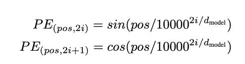
On Line 7, we build the positional_encoding function. This function takes the length of positions and the depth of each embedding. It computes the positional encoding suggested by Vaswani et al. (Attention Is All You Need). You can also see the formula for the encoding, as shown in Figure 1.

On Line 18, we divide the depth into two equal halves, one for the sine and the other for cosine frequencies. From Lines 21-26, we build the positions, depths, angleRates, and angleRads needed for the formula.

On Line 29, the entire positional encoding is built where we concatenate the sine and cosine outputs together; posEncoding is then returned on Line 30.

class PositionalEmbedding(Layer):
    def __init__(self, vocabSize, dModel, maximumPositionEncoding, **kwargs):
        """
        Args:
            vocabSize: The vocabulary size of the target or source dataset
            dModel: The dimension of the transformer model
            maximumPositionEncoding: The maximum length of a sentence in the dataset
        """
        super().__init__(**kwargs)

        # initialize an embedding layer
        self.embedding = Embedding(
            input_dim=vocabSize, output_dim=dModel, mask_zero=True
        )

        # initialize the positional encoding function
        self.posEncoding = positional_encoding(
            length=maximumPositionEncoding, depth=dModel
        )

        # define the dimensions of the model
        self.dModel = dModel

    def compute_mask(self, *args, **kwargs):
        # return the padding mask from the inputs
        return self.embedding.compute_mask(*args, **kwargs)

    def call(self, x):
        # get the length of the input sequence
        seqLen = tf.shape(x)[1]

        # embed the input and scale the embeddings
        x = self.embedding(x)
        x *= tf.math.sqrt(tf.cast(self.dModel, tf.float32))

        # add the positional encoding with the scaled embeddings
        x += self.posEncoding[tf.newaxis, :seqLen, :]

        # return the encoded input
        return x

It is always better to build a tf.keras.layers.Layer for custom layers that we need in our model. PositionalEmbedding is one such layer. We define the custom layer on Line 33.

We initialize the layer with an Embedding and a positional_encoding layer, as done on Lines 44-51. We also define the dimension of the model on Line 54.

Keras lets us expose a compute_mask method for the custom layer. We define this method on Line 56. For more information about padding and masking, one can read the official TensorFlow guide.

The call method accepts x as its input (Line 60). The inputs are first embedded (Line 65), then the positional encoding is added to the embedded inputs (Line 69), which is finally returned on Line 72.

---

Feed Forward

To build the feed-forward network module, as shown in the previous blog post, we open the feed_forward.py inside the pyimagesearch directory.

# import the necessary packages
from tensorflow.keras import Sequential
from tensorflow.keras.layers import Add, Dense, Dropout, Layer, LayerNormalization

On Lines 2 and 3, we import the necessary packages.

class FeedForward(Layer):
    def __init__(self, dff, dModel, dropoutRate=0.1, **kwargs):
        """
        Args:
            dff: Intermediate dimension for the feed forward network
            dModel: The dimension of the transformer model
            dropOutRate: Rate for dropout layer
        """
        super().__init__(**kwargs)

        # initialize the sequential model of dense layers
        self.seq = Sequential(
            [
                Dense(units=dff, activation="relu"),
                Dense(units=dModel),
                Dropout(rate=dropoutRate),
            ]
        )

        # initialize the addition layer and layer normalization layer
        self.add = Add()
        self.layernorm = LayerNormalization()

    def call(self, x):
        # add the processed input and original input
        x = self.add([x, self.seq(x)])

        # apply layer norm on the residual and return it
        x = self.layernorm(x)
        return x

On Line 6, we define the custom layer FeedForward. The layer is initialized with a tf.keras.Sequential module (Lines 17-23), an Add layer (Line 26), and a LayerNormalization layer (Line 27). The Sequential model has a stack of Dense and Dropout layers. This is nothing but our feed-forward network that goes into the transformer sublayer.

The call method (Line 29) accepts x as its input. The inputs are passed through the sequential model and added with the original input as a residual connection on Line 31. The processed sublayer output is then passed through the layernorm layer on Line 34.

The output is then returned on Line 35.

---

Rate Schedule

To build the Learning Rate Scheduler module, we open the rate_schedule.py file inside the pyimagesearch directory.

# import the necessary packages
import tensorflow as tf
from tensorflow.keras.optimizers.schedules import LearningRateSchedule

On Lines 2 and 3, we import the necessary packages important for the rate schedule.

class CustomSchedule(LearningRateSchedule):
    def __init__(self, dModel, warmupSteps=4000):
        super().__init__()

        # define the dmodel and warmup steps
        self.dModel = dModel
        self.dModel = tf.cast(self.dModel, tf.float32)
        self.warmupSteps = warmupSteps

    def __call__(self, step):
        # build the custom schedule logic
        step = tf.cast(step, dtype=tf.float32)
        arg1 = tf.math.rsqrt(step)
        arg2 = step * (self.warmupSteps**-1.5)

        return tf.math.rsqrt(self.dModel) * tf.math.minimum(arg1, arg2)

On Line 6, we build the custom LearningRateSchedule implemented in the paper. We name it CustomSchedule (with a lot of creativity).

On Lines 7-13, we initialize the module with the necessary arguments. We define the dimension of the model and the number of warmup steps on Lines 11 and 13, respectively.

The logic for the custom schedule can be seen as shown in Figure 2. We have implemented the same logic in TensorFlow in the __call__ method (from Lines 15-21).

---

Loss Accuracy

We build the module for defining the metrics inside loss_accuracy.py under the pyimagesearch directory.

# import the necessary packages
import tensorflow as tf
from tensorflow.keras.losses import SparseCategoricalCrossentropy

On Lines 2 and 3, we import the necessary packages.

def masked_loss(label, prediction):
    # mask positions where the label is not equal to 0
    mask = label != 0

    # build the loss object and apply it to the labels
    lossObject = SparseCategoricalCrossentropy(from_logits=True, reduction="none")
    loss = lossObject(label, prediction)

    # mask the loss
    mask = tf.cast(mask, dtype=loss.dtype)
    loss *= mask

    # average the loss over the batch and return it
    loss = tf.reduce_sum(loss) / tf.reduce_sum(mask)
    return loss

On Line 6, we build our masked_loss function. It accepts the true label and the prediction from our model as inputs.

We first build the mask on Line 8. The mask is everywhere the label is not equal to 0. With SparseCategoricalCrossentropy as our loss object, we compute the raw loss excluding the masks on Lines 11 and 12.

The raw loss is then multiplied with the boolean mask to get the masked loss on Lines 15 and 16. On Line 19, we average the masked loss and return it on Line 20.

def masked_accuracy(label, prediction):
    # mask positions where the label is not equal to 0
    mask = label != 0

    # get the argmax from the logits
    prediction = tf.argmax(prediction, axis=2)

    # cast the label into the prediction datatype
    label = tf.cast(label, dtype=prediction.dtype)

    # calculate the matches
    match = label == prediction
    match = match & mask

    # cast the match and masks
    match = tf.cast(match, dtype=tf.float32)
    mask = tf.cast(mask, dtype=tf.float32)

    # average the match over the batch and return it
    match = tf.reduce_sum(match) / tf.reduce_sum(mask)
    return match

On Line 23, we define our custom masked_accuracy function. This will be our custom metric while we train the transformer model.

On Line 25, we build the boolean mask. The mask is then typecast to the data type of the prediction on Line 31.

Lines 34 and 35 compute the matches (required to compute accuracy) and then apply the mask to get the masked matches.

Lines 38 and 39 typecast the matches and the masks. On Line 42, we average the masked matches and return them on Line 43.

---

Encoder

In Figure 3, we can see the encoder highlighted in the Transformer Architecture. As shown in Figure 3, the encoder is a stack of N identical layers. Each layer is composed of two sublayers.

The first is a multi-head self-attention mechanism, and the second is a simple, position-wise, fully connected feed-forward network.

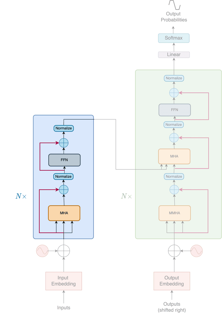
Vaswani et al. (2017) also employ residual connections and a normalization operation around the two sublayers.

We build the encoder module inside the pyimagesearch directory and name it encoder.py.

# import the necessary packages
import tensorflow as tf
from tensorflow.keras.layers import Dropout, Layer

from .attention import GlobalSelfAttention
from .feed_forward import FeedForward
from .positional_encoding import PositionalEmbedding

On Lines 2 and 7, we import the necessary packages.

class EncoderLayer(Layer):
    def __init__(self, dModel, numHeads, dff, dropOutRate=0.1, **kwargs):
        """
        Args:
            dModel: The dimension of the transformer module
            numHeads: Number of heads of the multi head attention module in the encoder layer
            dff: The intermediate dimension size in the feed forward network
            dropOutRate: The rate of dropout layer
        """
        super().__init__(**kwargs)

        # define the Global Self Attention layer
        self.globalSelfAttention = GlobalSelfAttention(
            num_heads=numHeads,
            key_dim=dModel // numHeads,
            dropout=dropOutRate,
        )

        # initialize the pointwise feed forward sublayer
        self.ffn = FeedForward(dff=dff, dModel=dModel, dropoutRate=dropOutRate)

    def call(self, x):
        # apply global self attention to the inputs
        x = self.globalSelfAttention(x)

        # apply feed forward network and return the outputs
        x = self.ffn(x)
        return x

An encoder is a stack of encoder layers. Here, on Line 10, we define the encoder layer that holds the two sublayers, namely global self-attention (Lines 22-26) and the feed-forward layer (Line 29).

The call method is simple. On Line 33, we apply the global self-attention on the inputs to the encoder layer. On Line 36, we process the attended outputs with the point-wise feed-forward network.

The output of the encoder layer is then returned on Line 37.

class Encoder(Layer):
    def __init__(
        self,
        numLayers,
        dModel,
        numHeads,
        sourceVocabSize,
        maximumPositionEncoding,
        dff,
        dropOutRate=0.1,
        **kwargs
    ):
        """
        Args:
            numLayers: The number of encoder layers in the encoder
            dModel: The dimension of the transformer module
            numHeads: Number of heads of multihead attention layer in each encoder layer
            sourceVocabSize: The source vocabulary size
            maximumPositionEncoding: The maximum number of tokens in a sentence in the source dataset
            dff: The intermediate dimension of the feed forward network
            dropOutRate: The rate of dropout layer
        """
        super().__init__(**kwargs)

        # define the dimension of the model and the number of encoder layers
        self.dModel = dModel
        self.numLayers = numLayers

        # initialize the positional embedding layer
        self.positionalEmbedding = PositionalEmbedding(
            vocabSize=sourceVocabSize,
            dModel=dModel,
            maximumPositionEncoding=maximumPositionEncoding,
        )

        # define a stack of encoder layers
        self.encoderLayers = [
            EncoderLayer(
                dModel=dModel, dff=dff, numHeads=numHeads, dropOutRate=dropOutRate
            )
            for _ in range(numLayers)
        ]

        # initialize a dropout layer
        self.dropout = Dropout(rate=dropOutRate)

    def call(self, x):
        # apply positional embedding to the source token ids
        x = self.positionalEmbedding(x)

        # apply dropout to the embedded inputs
        x = self.dropout(x)

        # iterate over the stacks of encoder layer
        for encoderLayer in self.encoderLayers:
            x = encoderLayer(x=x)

        # return the output of the encoder
        return x

On Lines 40-51, we define our Encoder layer. The encoder, as stated above, consists of a stack of encoder layers. To make the encoder self-sufficient, we also add the positional encoding layer inside the encoder itself.

On Lines 65 and 66, we define the dimension of the encoder and the number of encoder layers that build the encoder.

Lines 76-81 build the stack of encoder layers. On Line 84, we initialize a Dropout layer to regularize the model.

The call method of the layer accepts x as input. First, we apply the positional encoding layer on the input, as seen on Line 88. Then the embeddings are sent to the Dropout layer on Line 91. The processed input is then iterated over the encoder layers on Lines 94 and 95. The output of the encoder is then returned on Line 98.

---

Decoder

Next, in Figure 4, we can see the decoder being highlighted in the Transformer architecture.

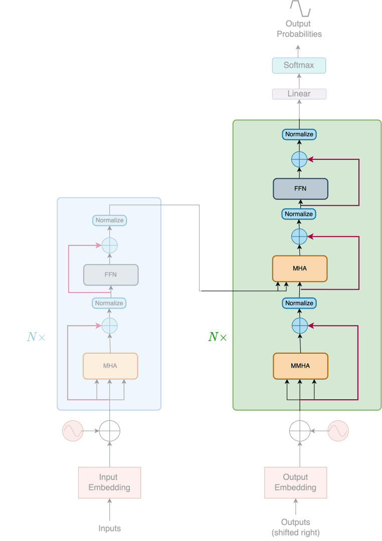
In addition to the two sublayers in each encoder layer, the decoder inserts a third sublayer, which performs multi-head attention over the output of the encoder stack.

The decoder also has residual connections and a normalization operation around the three sublayers. Notice that the first sublayer of the decoder is a masked multi-head attention layer instead of a multi-head attention layer.

We build the decoder module inside the pyimagesearch and name it decoder.py.

# import the necessary packages
import tensorflow as tf
from tensorflow.keras.layers import Dropout, Layer

from pyimagesearch.attention import CausalSelfAttention, CrossAttention

from .feed_forward import FeedForward
from .positional_encoding import PositionalEmbedding

On Lines 2-8, we import the necessary packages.

class DecoderLayer(Layer):
    def __init__(self, dModel, numHeads, dff, dropOutRate=0.1, **kwargs):
        """
        Args:
            dModel: The dimension of the transformer module
            numHeads: Number of heads of the multi head attention module in the encoder layer
            dff: The intermediate dimension size in the feed forward network
            dropOutRate: The rate of dropout layer
        """
        super().__init__(**kwargs)

        # initialize the causal attention module
        self.causalSelfAttention = CausalSelfAttention(
            num_heads=numHeads,
            key_dim=dModel // numHeads,
            dropout=dropOutRate,
        )

        # initialize the cross attention module
        self.crossAttention = CrossAttention(
            num_heads=numHeads,
            key_dim=dModel // numHeads,
            dropout=dropOutRate,
        )

        # initialize a feed forward network
        self.ffn = FeedForward(
            dff=dff,
            dModel=dModel,
            dropoutRate=dropOutRate,
        )

    def call(self, x, context):
        x = self.causalSelfAttention(x=x)
        x = self.crossAttention(x=x, context=context)

        # get the attention scores for plotting later
        self.lastAttentionScores = self.crossAttention.lastAttentionScores

        # apply feedforward network to the outputs and return it
        x = self.ffn(x)
        return x

The decoder is a stack of individual decoder layers. On Line 11, we define the custom DecoderLayer. On Lines 23-27, we define the CausalSelfAttention layer. This layer is the first sublayer in the decoder layer. This provides the causal masking to the target inputs.

On Lines 30-34, we define the CrossAttention layer. This will process the output of the CausalAttention layer and the Encoder outputs. The term cross comes from the inputs to this sublayer from the decoder and the encoder together.

On Lines 37-41, we define the FeedForward layer.

The call method of the custom layer is defined on Line 43. It accepts x and context as inputs. On Lines 44 and 45, the inputs are processed by the causal and cross-attention layers, respectively.

The attention scores are cached on Line 48. After that, we apply the feed-forward network on the processed output on Line 51. The output of the custom decoder layer is then returned on Line 52.

class Decoder(Layer):
    def __init__(
        self,
        numLayers,
        dModel,
        numHeads,
        targetVocabSize,
        maximumPositionEncoding,
        dff,
        dropOutRate=0.1,
        **kwargs
    ):
        """
        Args:
            numLayers: The number of encoder layers in the encoder
            dModel: The dimension of the transformer module
            numHeads: Number of heads of multihead attention layer in each encoder layer
            targetVocabSize: The target vocabulary size
            maximumPositionEncoding: The maximum number of tokens in a sentence in the source dataset
            dff: The intermediate dimension of the feed forward network
            dropOutRate: The rate of dropout layer
        """
        super().__init__(**kwargs)

        # define the dimension of the model and the number of decoder layers
        self.dModel = dModel
        self.numLayers = numLayers

        # initialize the positional embedding layer
        self.positionalEmbedding = PositionalEmbedding(
            vocabSize=targetVocabSize,
            dModel=dModel,
            maximumPositionEncoding=maximumPositionEncoding,
        )

        # define a stack of decoder layers
        self.decoderLayers = [
            DecoderLayer(
                dModel=dModel, dff=dff, numHeads=numHeads, dropOutRate=dropOutRate
            )
            for _ in range(numLayers)
        ]

        # initialize a dropout layer
        self.dropout = Dropout(rate=dropOutRate)

    def call(self, x, context):
        # apply positional embedding to the target token ids
        x = self.positionalEmbedding(x)

        # apply dropout to the embedded targets
        x = self.dropout(x)

        # iterate over the stacks of decoder layer
        for decoderLayer in self.decoderLayers:
            x = decoderLayer(x=x, context=context)

        # get the attention scores and cache it
        self.lastAttentionScores = self.decoderLayers[-1].lastAttentionScores

        # return the output of the decoder
        return x

We define the Decoder layer on Lines 55-66. On Lines 80 and 81, we define the dimension of the decoder model and the number of decoder layers used in the decoder.

Lines 84-88 define the positional encoding layer. On Lines 91-96, we define the stack of decoder layers for the decoder. We also define a Dropout layer on Line 99.

The call method is defined on Line 101. It accepts x and context as inputs. On Line 103, we first pass the x tokens through the positionalEmbedding layer to embed it. On Line 106, we apply dropout to the embeddings to regularize the model.

We iterate over the stack of decoder layers and apply it to the embeddings and context inputs, as shown on Lines 109 and 110. We also cache the last attention scores on Line 113.

The output of the decoder is returned on Line 116.

---

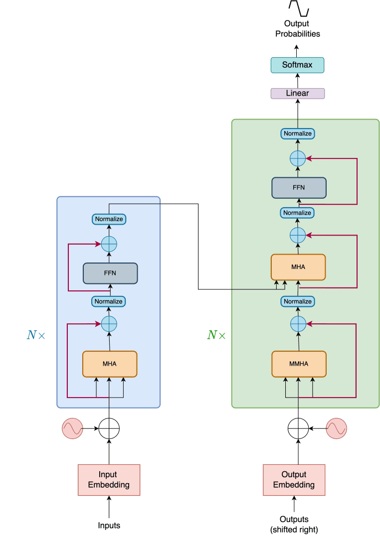
Transformer

Finally, all the modules and components are ready to build the entire transformer architecture. Let us look at Figure 5, where we see the entire Architecture.

We build the entire module in transformer.py inside the pyimagesearch directory.

# import the necessary packages
import tensorflow as tf
from tensorflow.keras import Model
from tensorflow.keras.layers import Dense
from tensorflow.keras.metrics import Mean

from pyimagesearch.decoder import Decoder
from pyimagesearch.encoder import Encoder

Lines 2-8 import the necessary packages.

class Transformer(Model):
    def __init__(
        self,
        encNumLayers,
        decNumLayers,
        dModel,
        numHeads,
        dff,
        sourceVocabSize,
        targetVocabSize,
        maximumPositionEncoding,
        dropOutRate=0.1,
        **kwargs
    ):
        """
        Args:
            encNumLayers: The number of encoder layers
            decNumLayers: The number of decoder layers
            dModel: The dimension of the transformer model
            numHeads: The number of multi head attention module for the encoder and decoder layers
            dff: The intermediate dimension of the feed forward network
            sourceVocabSize: The source vocabulary size
            targetVocabSize: The target vocabulary size
            maximumPositionEncoding: The maximum token length in the dataset
            dropOutRate: The rate of dropout layers
        """
        super().__init__(**kwargs)

        # initialize the encoder and the decoder layers
        self.encoder = Encoder(
            numLayers=encNumLayers,
            dModel=dModel,
            numHeads=numHeads,
            sourceVocabSize=sourceVocabSize,
            maximumPositionEncoding=maximumPositionEncoding,
            dff=dff,
            dropOutRate=dropOutRate,
        )
        self.decoder = Decoder(
            numLayers=decNumLayers,
            dModel=dModel,
            numHeads=numHeads,
            targetVocabSize=targetVocabSize,
            maximumPositionEncoding=maximumPositionEncoding,
            dff=dff,
            dropOutRate=dropOutRate,
        )

        # define the final layer of the transformer
        self.finalLayer = Dense(units=targetVocabSize)

    def call(self, inputs):
        # get the source and the target from the inputs
        (source, target) = inputs

        # get the encoded representation from the source inputs and the
        # decoded representation from the encoder outputs and target inputs
        encoderOutput = self.encoder(x=source)
        decoderOutput = self.decoder(x=target, context=encoderOutput)

        # apply a dense layer to the decoder output to formulate the logits
        logits = self.finalLayer(decoderOutput)

        # drop the keras mask, so it doesn't scale the losses/metrics.
        try:
            del logits._keras_mask
        except AttributeError:
            pass

        # return the final logits
        return logits

We have already defined the Decoder and the Encoder custom layers. It is time we put everything together and build our Transformer model.

Notice how we define a custom tf.keras.Model named Transformer on Line 11. The arguments needed to build the Transformer are mentioned on Lines 12-24.

From Lines 40-57, we define the Encoder and the Decoder. On Line 60, we initialize the final dense layer that computes the logits.

The call method of the model is defined on Line 62. The inputs are the source and target tokens. We first segregate the two on Line 64. On Line 68, we apply the encoder on the source tokens to get the encoder representation. Next, on Line 69, we apply the decoder on the target tokens and the encoder representations.

To compute the logits, we apply the final dense layer on the decoder output, as shown on Line 72. We then remove the attached keras mask on Lines 75-78. We then return the logits on Line 81.

---

Translator

However, there are a few more components that we need to build to train and test the entire architecture. The first is a translator module we will need at inference to perform neural machine translation.

We build the translator module inside the pyimagesearch directory and name it translate.py.

import numpy as np
import tensorflow as tf
from tensorflow.keras.layers import StringLookup

On Lines 1-3, we import the necessary packages.

class Translator(tf.Module):
    def __init__(
        self,
        sourceTextProcessor,
        targetTextProcessor,
        transformer,
        maxLength
    ):
        # initialize the source text processor
        self.sourceTextProcessor = sourceTextProcessor

        # initialize the target text processor and a string from
        # index string lookup layer for the target ids
        self.targetTextProcessor = targetTextProcessor
        self.targetStringFromIndex = StringLookup(
            vocabulary=targetTextProcessor.get_vocabulary(),
            mask_token="",
            invert=True
        )

        # initialize the pre-trained transformer model
        self.transformer = transformer

        self.maxLength = maxLength

The Transformer model, after being trained, needs an API to infer. We would need a custom translator that uses the trained transformer model and gives us results in human-readable strings.

On Line 5, we define our custom tf.Module names Translator, which would translate the source sentence to the target sentence using the pre-trained Transformer model. On Line 14, we define the source text processor.

On Lines 18-23, we define the target text processor and a string lookup layer. The string lookup is important to get the string from the token ids.

Line 26 defined the pretrained transformer model. Line 28 defines the maximum length of translated sentences.

    def tokens_to_text(self, resultTokens):
        # decode the token from index to string
        resultTextTokens = self.targetStringFromIndex(resultTokens)

        # format the result text into a human readable format
        resultText = tf.strings.reduce_join(
            inputs=resultTextTokens, axis=1, separator=" "
        )
        resultText = tf.strings.strip(resultText)

        # return the result text
        return resultText

The tokens_to_text method is necessary to turn the token ids into strings. It accepts resultTokens as input (Line 30).

On Line 32, we decode the token from the index to string. This is where the string lookup layer is utilized. Lines 35-38 take care of joining the strings and stripping off the white spaces. This is necessary to turn the output strings into human-readable sentences.

The processed text is then returned on Line 41.

    @tf.function(input_signature=[tf.TensorSpec(shape=[], dtype=tf.string)])
    def __call__(self, sentence):
        # the input sentence is a string of source language
        # apply the source text processor on the list of source sentences
        sentence = self.sourceTextProcessor(sentence[tf.newaxis])

        encoderInput = sentence

        # apply the target text processor on an empty sentence
        # this will create the start and end tokens
        startEnd = self.targetTextProcessor([""])[0] # 0 index is to index the only batch

        # grab the start and end tokens individually
        startToken = startEnd[0][tf.newaxis]
        endToken = startEnd[1][tf.newaxis]

        # build the output array
        outputArray = tf.TensorArray(dtype=tf.int64, size=0, dynamic_size=True)
        outputArray = outputArray.write(index=0, value=startToken)

        # iterate over the maximum length and get the output ids
        for i in tf.range(self.maxLength):
            # transpose the output array stack
            output = tf.transpose(outputArray.stack())

            # get the predictions from the transformer and
            # grab the last predicted token
            predictions = self.transformer([encoderInput, output], training=False)
            predictions = predictions[:, -1:, :] # (bsz, 1, vocabSize)

            # get the predicted id from the predictions using argmax and
            # write the predicted id into the output array
            predictedId = tf.argmax(predictions, axis=-1)
            outputArray = outputArray.write(i+1, predictedId[0])

            # if the predicted id is the end token stop iteration
            if predictedId == endToken:
                break

        output = tf.transpose(outputArray.stack())
        text = self.tokens_to_text(output)

        return text

We now define the __call__ method of the Translator on Lines 43 and 44. The input sentence is a string of source language. We apply the source text processor on the list of source sentences on Line 47.

The encoder input is the tokenized input, as shown on Line 49. On Lines 51-53, we apply the target text processor on an empty sentence, creating the start and end tokens. The start and end tokens are segregated on Lines 56 and 57.

We build the output array, tf.TensorArray, on Lines 60 and 61. We now iterate over the maximum number of tokens generated and generate the output token ids from the pre-trained Transformer model (Lines 64-80). On Line 66, we transpose the output array stack. On Lines 70 and 71, we get the predictions from the transformer and grab the last predicted token.

We get the predicted id from the predictions using tf.argmax and write the predicted id into the output array on Lines 75 and 76. A condition to stop the iteration is provided on Lines 79 and 80. The condition is that the predicted token should match the end token.

We then apply the tokens_to_text method to the output array and get the resulting text in strings on Lines 82 and 83. This resulting text is returned on Line 85.

---

Training

We assemble all the parts to train the transformer architecture for the Neural Machine Translation task. The training module is built inside train.py.

# USAGE
# python train.py

# setting seed for reproducibility
import sys
import tensorflow as tf

from pyimagesearch.loss_accuracy import masked_accuracy, masked_loss
from pyimagesearch.translate import Translator

tf.keras.utils.set_random_seed(42)
from tensorflow.keras.layers import TextVectorization
from tensorflow.keras.optimizers import Adam

from pyimagesearch import config
from pyimagesearch.dataset import (
    load_data,
    make_dataset,
    splitting_dataset,
    tf_lower_and_split_punct,
)
from pyimagesearch.rate_schedule import CustomSchedule
from pyimagesearch.transformer import Transformer

On Lines 5-23, we define the imports and set the random seed for reproducibility.

# load data from disk
print(f"[INFO] loading data from {config.DATA_FNAME}...")
(source, target) = load_data(fname=config.DATA_FNAME)

Lines 26 and 27 load the data using the load_data method.

# split the data into training, validation, and test set
print("[INFO] splitting the dataset into train, val, and test...")
(train, val, test) = splitting_dataset(source=source, target=target

A dataset needs to be split into train, val, and test. Lines 30 and 31 help in just that. The dataset is sent over to the splitting_dataset function, which splits it into the respective data splits.

# create source text processing layer and adapt on the training
# source sentences
print("[INFO] adapting the source text processor on the source dataset...")
sourceTextProcessor = TextVectorization(
    standardize=tf_lower_and_split_punct, max_tokens=config.SOURCE_VOCAB_SIZE
)
sourceTextProcessor.adapt(train[0])

Lines 35-39 create the source text processor, a TextVectorization layer, and adapt it on the source training dataset.

# create target text processing layer and adapt on the training
# target sentences
print("[INFO] adapting the target text processor on the target dataset...")
targetTextProcessor = TextVectorization(
    standardize=tf_lower_and_split_punct, max_tokens=config.TARGET_VOCAB_SIZE
)
targetTextProcessor.adapt(train[1])

Lines 43-47 create the target text processor, a TextVectorization layer, and adapt to the target training dataset.

# build the TensorFlow data datasets of the respective data splits
print("[INFO] building TensorFlow Data input pipeline...")
trainDs = make_dataset(
    splits=train,
    batchSize=config.BATCH_SIZE,
    train=True,
    sourceTextProcessor=sourceTextProcessor,
    targetTextProcessor=targetTextProcessor,
)
valDs = make_dataset(
    splits=val,
    batchSize=config.BATCH_SIZE,
    train=False,
    sourceTextProcessor=sourceTextProcessor,
    targetTextProcessor=targetTextProcessor,
)
testDs = make_dataset(
    splits=test,
    batchSize=config.BATCH_SIZE,
    train=False,
    sourceTextProcessor=sourceTextProcessor,
    targetTextProcessor=targetTextProcessor,
)

Lines 50-71 builds the tf.data.Dataset pipeline using the make_dataset function.

# build the transformer model
print("[INFO] building the transformer model...")
transformerModel = Transformer(
    encNumLayers=config.ENCODER_NUM_LAYERS,
    decNumLayers=config.DECODER_NUM_LAYERS,
    dModel=config.D_MODEL,
    numHeads=config.NUM_HEADS,
    dff=config.DFF,
    sourceVocabSize=config.SOURCE_VOCAB_SIZE,
    targetVocabSize=config.TARGET_VOCAB_SIZE,
    maximumPositionEncoding=config.MAX_POS_ENCODING,
    dropOutRate=config.DROP_RATE,
)

We build our Transformer model on Lines 74-85.

# compile the model
print("[INFO] compiling the transformer model...")
learningRate = CustomSchedule(dModel=config.D_MODEL)
optimizer = Adam(learning_rate=learningRate, beta_1=0.9, beta_2=0.98, epsilon=1e-9)
transformerModel.compile(
    loss=masked_loss, optimizer=optimizer, metrics=[masked_accuracy]
)

We compile the model with the custom optimizer with CustomSchedule and the masked_loss and masked_accuracy functions on Lines 88-93.

# fit the model on the training dataset
transformerModel.fit(
    trainDs,
    epochs=config.EPOCHS,
    validation_data=valDs,
)

Using trainDs we fit the model on Lines 96-100. Here, we use the efficient and elegant Model.fit API provided by Keras. We also validate the training pipeline by providing valDs to the fit method.

# infer on a sentence
translator = Translator(
    sourceTextProcessor=sourceTextProcessor,
    targetTextProcessor=targetTextProcessor,
    transformer=transformerModel,
    maxLength=50,
)

# serialize and save the translator
print("[INFO] serialize the inference translator to disk...")
tf.saved_model.save(
    obj=translator,
    export_dir="translator",
)

We build Translator for inference and save it to disk on Lines 103-115.

The following is the output of the training script for a mere 25 epochs.

$ python train.py
[INFO] loading data from fra.txt...
[INFO] splitting the dataset into train, val, and test...
[INFO] adapting the source text processor on the source dataset...
[INFO] adapting the target text processor on the target dataset...
[INFO] building TensorFlow Data input pipeline...
[INFO] building the transformer model...
[INFO] compiling the transformer model...
Epoch 1/25
309/309 [==============================] - 85s 207ms/step - loss: 7.1164 - masked_accuracy: 0.2238 - val_loss: 4.8327 - val_masked_accuracy: 0.3452
Epoch 2/25
309/309 [==============================] - 61s 197ms/step - loss: 3.9636 - masked_accuracy: 0.4155 - val_loss: 3.0660 - val_masked_accuracy: 0.5020
.
.
.
Epoch 24/25
309/309 [==============================] - 61s 195ms/step - loss: 0.2388 - masked_accuracy: 0.9185 - val_loss: 1.0194 - val_masked_accuracy: 0.8032
Epoch 25/25
309/309 [==============================] - 61s 195ms/step - loss: 0.2276 - masked_accuracy: 0.9217 - val_loss: 1.0323 - val_masked_accuracy: 0.8036
[INFO] serialize the inference translator to disk...

---

Inference

Now for the interesting part. We will test how well our Transformer performs the task of machine translation. We build the inference script inside inference.py.

# USAGE
# python inference.py -s "input sentence"

We define the usage of the inference script on Lines 1 and 2.

# import the necessary packages
import tensorflow_text as tf_text # this is a no op import important for op registry
import tensorflow as tf
import argparse

We import the necessary packages on Lines 5-7.

# construct the argument parse and parse the arguments
ap = argparse.ArgumentParser()
ap.add_argument("-s", "--sentence", required=True,
	help="input english sentence")
args = vars(ap.parse_args())

We construct the argument parse and parse the arguments on Lines 10-13.

# convert the input english sentence to a constant tensor
sourceText = tf.constant(args["sentence"])

Line 16 converts the input source sentence to a tf.Tensor. This is essential for the translator, as it accepts tf.Tensor and not strings.

# load the translator model from disk
print("[INFO] loading the translator model from disk...")
translator = tf.saved_model.load("translator")

We now load the saved Translator module from disk on Lines 19 and 20.

# perform inference and display the result
print("[INFO] translating english sentence to french...")
result = translator(sentence=sourceText)

translatedText = result.numpy()[0].decode()
print("[INFO] english sentence: {}".format(args["sentence"]))
print("[INFO] french translation: {}".format(translatedText))

On Lines 23-28, we then perform the inference on the Translator module and display the result on the terminal.

The following output shows the inference on translating an English sentence to French.

$ python inference.py -s "i am hungry, let's get some food"

[INFO] loading the translator model from disk...
[INFO] translating english sentence to french...
[INFO] english sentence: i am hungry, let's get some food
[INFO] french translation: [START] jai faim , allons chercher de la nourriture . [END]

You can see and interact directly with the model through the Hugging Face Spaces right here:

---

---

Summary

The Transformer blog post is a culmination of multiple series at PyImageSearch. We begin at the very beginning with letters and words (tokens) and then build representations of these tokens. We also use these representations to find similarities between tokens and embed them in a high-dimensional space.

The same embeddings are also passed into sequential models (RNNs) that can process sequential data. Those models are used to build context and, ingeniously, attend to parts of the input sentence that are useful to the output sentence in translation. This entire narrative has spanned multiple blog posts, and we are very thankful to our readers who have been on this journey with us.

But as they say, “Every ending is a new beginning,” while the journey of the Transformer architecture and application to NLP ends here, we are left with some burning questions.

• How to apply this to images?
• How can we scale this?
• Can we build Transformers for every kind of modality out there?

Now, these questions need their own blog posts, and some need their own series! So, let us know what topic you want us to cover next:

Tweet @pyimagesearch OR email ask.me@pyimagesearch.com

---

References

We used the following references for the entire series:

• Neural machine translation with a Transformer and Keras
• Lecture 13: Attention
• Vaswani et al., 2017, “Attention Is All You Need”
• Manim Community

---

Citation Information

A. R. Gosthipaty and R. Raha. “A Deep Dive into Transformers with TensorFlow and Keras: Part 3,” PyImageSearch, P. Chugh, S. Huot, K. Kidriavsteva, and A. Thanki, eds., 2022, https://pyimg.co/9nozd

@incollection{ARG-RR_2022_DDTFK3,
  author = {Aritra Roy Gosthipaty and Ritwik Raha},
  title = {A Deep Dive into Transformers with {TensorFlow} and {K}eras: Part 3},
  booktitle = {PyImageSearch},
  editor = {Puneet Chugh and Susan Huot and Kseniia Kidriavsteva and Abhishek Thanki},
  year = {2022},
  note = {https://pyimg.co/9nozd},
}

---

---

To download the source code to this post (and be notified when future tutorials are published here on PyImageSearch), simply enter your email address in the form below!