OpenCV Edge Detection ( cv2.Canny )

In this tutorial, you will learn how to perform edge detection using OpenCV and the Canny edge detector.

Previously, we discussed image gradients and how they are one of the fundamental building blocks of computer vision and image processing.

A diverse image dataset is vital for understanding edge detection using the Canny Edge Detector. It provides a broad perspective on how edges can be detected in different types of images and under various conditions.

Roboflow has free tools for each stage of the computer vision pipeline that will streamline your workflows and supercharge your productivity.

Sign up or Log in to your Roboflow account to access state of the art dataset libaries and revolutionize your computer vision pipeline.

You can start by choosing your own datasets or using our PyimageSearch’s assorted library of useful datasets.

Bring data in any of 40+ formats to Roboflow, train using any state-of-the-art model architectures, deploy across multiple platforms (API, NVIDIA, browser, iOS, etc), and connect to applications or 3rd party tools.

Today, we are going to see just how important image gradients are; specifically, by examining the Canny edge detector.

The Canny edge detector is arguably the most well known and the most used edge detector in all of computer vision and image processing. While the Canny edge detector is not exactly “trivial” to understand, we’ll break down the steps into bite-sized pieces so we can understand what is going on under the hood.

Fortunately for us, since the Canny edge detector is so widely used in almost all computer vision applications, OpenCV has already implemented it for us in the cv2.Canny function.

We’ll also explore how to use this function to detect edges in images of our own.

To learn how to perform edge detection with OpenCV and the Canny edge detector, just keep reading.

OpenCV Edge Detection ( cv2.Canny )

In the first part of this tutorial, we’ll discuss what edge detection is and why we use it in our computer vision and image processing applications.

We’ll then review the types of edges in an image, including:

• Step edges
• Ramp edges
• Ridge edges
• Roof edges

With these reviewed we can discuss the four step process to Canny edge detection

1. Gaussian smoothing
2. Computing the gradient magnitude and orientation
3. Non-maxima suppression
4. Hysteresis thresholding

We’ll then learn how to implement the Canny edge detector using OpenCV and the cv2.Canny function.

What is edge detection?

As we discovered in the previous blog post on image gradients, the gradient magnitude and orientation allow us to reveal the structure of objects in an image.

However, for the process of edge detection, the gradient magnitude is extremely sensitive to noise.

For example, let’s examine the gradient representation of the following image:

On the left, we have our original input image of a frontside and backside. And on the right, we have the image gradient representation.

As you can see, the gradient representation is a bit noisy. Sure, we have been able to detect the actual outline of the pills. But we’re also left with a lot of “noise” inside the pills itself representing the pill imprint.

So what if we wanted to detect just the outline of the pills?

That way, if we had just the outline, we could extract the pills from the image using something like contour detection. Wouldn’t that be nice?

Unfortunately, simple image gradients are not going to allow us to (easily) achieve our goal.

Instead, we’ll have to use the image gradients as building blocks to create a more robust method to detect edges — the Canny edge detector.

The Canny edge detector

The Canny edge detector is a multi-step algorithm used to detect a wide range of edges in images. The algorithm itself was introduced by John F. Canny in his 1986 paper, A Computational Approach to Edge Detection.

If you look inside many image processing projects, you’ll most likely see the Canny edge detector being called somewhere in the source code. Whether we are finding the distance from our camera to an object, building a document scanner, or finding a Game Boy screen in an image, the Canny edge detector will often be found as an important preprocessing step.

More formally, an edge is defined as discontinuities in pixel intensity, or more simply, a sharp difference and change in pixel values.

Here is an example of applying the Canny edge detector to detect edges in our pill image from above:

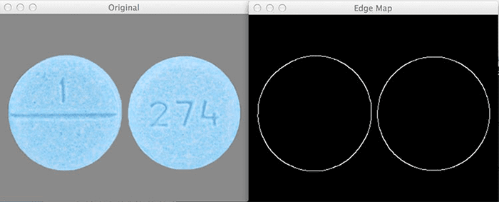
On the left, we have our original input image. And on the right, we have the output, or what is commonly called the edge map. Notice how we have only the outlines of the pill as a clear, thin white line — there is no longer any “noise” inside the pills themselves.

Before we dive deep into the Canny edge detection algorithm, let’s start by looking what types of edges there are in images:

Step edge

A step edge forms when there is an abrupt change in pixel intensity from one side of the discontinuity to the other. Take a look at the following graph for an example of a step edge:

As the name suggests, the graph actually looks like a step — there is a sharp step in the graph, indicating an abrupt change in pixel value. These types of edges tend to be easy to detect.

Ramp edge

A ramp edge is like a step edge, only the change in pixel intensity is not instantaneous. Instead, the change in pixel value occurs a short, but finite distance.

Here, we can see an edge that is slowly “ramping” up in change, but the change in intensity is not immediate like in a step edge:

Ridge edge

A ridge edge is similar to combining two ramp edges, one bumped right against another. I like to think of ramp edges as driving up and down a large hill or mountain:

First, you slowly ascend the mountain. Then you reach the top where it levels out for a short period. And then you’re riding back down the mountain.

In the context of edge detection, a ramp edge occurs when image intensity abruptly changes, but then returns to the initial value after a short distance.

Roof edge

Lastly we have the roof edge, which is a type of ridge edge:

Unlike the ridge edge where there is a short, finite plateau at the top of the edge, the roof edge has no such plateau. Instead, we slowly ramp up on either side of the edge, but the very top is a pinnacle and we simply fall back down the bottom.

Canny edge detection in a nutshell

Now that we have reviewed the various types of edges in an image, let’s discuss the actual Canny edge detection algorithm, which is a multi-step process consisting of:

1. Applying Gaussian smoothing to the image to help reduce noise
2. Computing the and image gradients using the Sobel kernel
3. Applying non-maxima suppression to keep only the local maxima of gradient magnitude pixels that are pointing in the direction of the gradient
4. Defining and applying the and thresholds for Hysteresis thresholding

Let’s discuss each of these steps.

Step #1: Gaussian smoothing

This step is fairly intuitive and straightforward. As we learned from our tutorial on smoothing and blurring, smoothing an image allows us to ignore much of the detail and instead focus on the actual structure.

This also makes sense in the context of edge detection — we are not interested in the actual detail of the image. Instead, we want to apply edge detection to find the structure and outline of the objects in the image so we can further process them.

Step #2: Gradient magnitude and orientation

Now that we have a smoothed image, we can compute the gradient orientation and magnitude, just like we did in the previous post.

However, as we have seen, the gradient magnitude is quite susceptible to noise and does not make for the best edge detector. We need to add two more steps on to the process to extract better edges.

Step #3: Non-maxima suppression

Non-maxima suppression sounds like a complicated process, but it’s really not — it’s simply an edge thinning process.

After computing our gradient magnitude representation, the edges themselves are still quite noisy and blurred, but in reality there should only be one edge response for a given region, not a whole clump of pixels reporting themselves as edges.

To remedy this, we can apply edge thinning using non-maxima suppression. To apply non-maxima suppression we need to examine the gradient magnitude and orientation at each pixel in the image and:

• Compare the current pixel to the neighborhood surrounding it
• Determine in which direction the orientation is pointing:
  • If it’s pointing towards the north or south, then examine the north and south magnitude
  • If the orientation is pointing towards the east or west, then examine the east and west pixels
• If the center pixel magnitude is greater than both the pixels it is being compared to, then preserve the magnitude; otherwise, discard it

Some implementations of the Canny edge detector round the value of to either , , , or , and then use the rounded angle to compare not only the north, south, east, and west pixels, but also the corner top-left, top-right, bottom-right, and bottom-left pixels as well.

But, let’s keep things simple and view an example of applying non-maxima suppression for an angle of degrees:

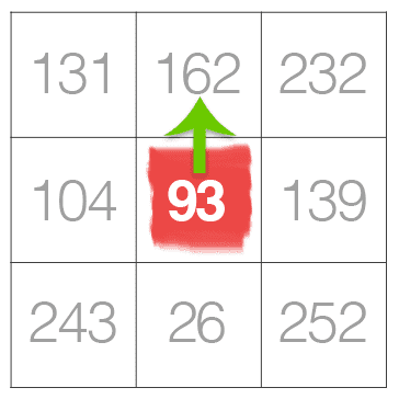
In the example above, we are going to pretend that the gradient orientation is (it’s actually not, but that’s okay, this is only an example).

Given that our gradient orientation is pointing north, we need to examine both the north and south pixels. The central pixel value of 93 is greater than the south value of 26, so we’ll discard the 26. However, examining the north pixel we see that the value is 162 — we’ll keep this value of 162 and suppress (i.e., set to 0) the value of 93 since 93 < 162.

Here’s another example of applying non-maxima suppression for when :

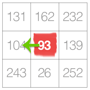
Notice how the central pixel is less than both the east and west pixels. According to our non-maxima suppression rules above (rule #3), we need to discard the pixel value of 93 and keep the east and west values of 104 and 139, respectively.

As you can see, non-maxima suppression for edge detection is not as hard as it seems!

Step #4: Hysteresis thresholding

Finally, we have the hysteresis thresholding step. Just like non-maxima suppression, it’s actually much easier than it sounds.

Even after applying non-maxima suppression, we may need to remove regions of an image that are not technically edges, but still respond as edges after computing the gradient magnitude and applying non-maximum suppression.

To ignore these regions of an image, we need to define two thresholds: and .

Any gradient value is sure to be an edge.

Any gradient value is definitely not an edge, so immediately discard these regions.

And any gradient value that falls into the range needs to undergo additional tests:

1. If the particular gradient value is connected to a strong edge (i.e., ), then mark the pixel as an edge.
2. If the gradient pixel is not connected to a strong edge, then discard it.

Hysteresis thresholding is actually better explained visually:

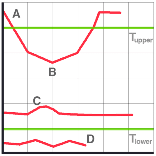
• At the top of the graph, we can see that A is a sure edge, since .
• B is also an edge, even though since it is connected to a sure edge, A.
• C is not an edge since and is not connected to a strong edge.
• Finally, D is not an edge since and is automatically discarded.

Setting these threshold ranges is not always a trivial process.

If the threshold range is too wide, then we’ll get many false edges instead of being about to find just the structure and outline of an object in an image.

Similarly, if the threshold range is too tight, we won’t find many edges at all and could be at risk of missing the structure/outline of the object entirely!

Later on in this series of posts, I’ll demonstrate how we can automatically tune these threshold ranges with practically zero effort. But for the time being, let’s see how edge detection is actually performed inside OpenCV.

Configuring your development environment

To follow this guide, you need to have the OpenCV library installed on your system.

Luckily, OpenCV is pip-installable:

$ pip install opencv-contrib-python

If you need help configuring your development environment for OpenCV, I highly recommend that you read my pip install OpenCV guide — it will have you up and running in a matter of minutes.

Having problems configuring your development environment?

All that said, are you:

• Short on time?
• Learning on your employer’s administratively locked system?
• Wanting to skip the hassle of fighting with the command line, package managers, and virtual environments?
• Ready to run the code right now on your Windows, macOS, or Linux system?

Then join PyImageSearch University today!

Gain access to Jupyter Notebooks for this tutorial and other PyImageSearch guides that are pre-configured to run on Google Colab’s ecosystem right in your web browser! No installation required.

And best of all, these Jupyter Notebooks will run on Windows, macOS, and Linux!

Project structure

Before we can compute edges using OpenCV and the Canny edge detector, let’s first review our project directory structure.

Be sure to access the “Downloads” section of this tutorial to retrieve the source code and example images:

$ tree . --dirsfirst
.
├── images
│   ├── clonazepam_1mg.png
│   └── coins.png
└── opencv_canny.py

1 directory, 3 files

We have a single Python script to review, opencv_canny.py, which will apply the Canny edge detector.

Inside the images directory, we have two example images that we’ll apply the Canny edge detector to.

Implementing the Canny edge detector with OpenCV

We are now ready to implement the Canny edge detector using OpenCV and the cv2.Canny function!

Open the opencv_cann.py file in your project structure and let’s review the code:

# import the necessary packages
import argparse
import cv2

# construct the argument parser and parse the arguments
ap = argparse.ArgumentParser()
ap.add_argument("-i", "--image", type=str, required=True,
	help="path to input image")
args = vars(ap.parse_args())

We start on Lines 2 and 3 by importing our required Python packages — we need only argparse for command line arguments and cv2 for our OpenCV bindings.

Command line arguments are parsed on Lines 6-9. A single switch is required, --image, which is the path to the input image we wish to apply edge detection to.

Let’s now load our image and preprocess it:

# load the image, convert it to grayscale, and blur it slightly
image = cv2.imread(args["image"])
gray = cv2.cvtColor(image, cv2.COLOR_BGR2GRAY)
blurred = cv2.GaussianBlur(gray, (5, 5), 0)

# show the original and blurred images
cv2.imshow("Original", image)
cv2.imshow("Blurred", blurred)

While Canny edge detection can be applied to an RGB image by detecting edges in each of the separate Red, Green, and Blue channels separately and combining the results back together, we almost always want to apply edge detection to a single channel, grayscale image (Line 13) — this ensures that there will be less noise during the edge detection process.

Secondly, while the Canny edge detector does apply blurring prior to edge detection, we’ll also want to (normally) apply extra blurring prior to the edge detector to further reduce noise and allow us to find the objects in an image (Line 14).

Lines 17 and 18 then display our original and blurred images on our screen.

We’re now ready to perform edge detection:

# compute a "wide", "mid-range", and "tight" threshold for the edges
# using the Canny edge detector
wide = cv2.Canny(blurred, 10, 200)
mid = cv2.Canny(blurred, 30, 150)
tight = cv2.Canny(blurred, 240, 250)

# show the output Canny edge maps
cv2.imshow("Wide Edge Map", wide)
cv2.imshow("Mid Edge Map", mid)
cv2.imshow("Tight Edge Map", tight)
cv2.waitKey(0)

Applying the cv2.Canny function to detect edges is performed on Lines 22-24.

The first parameter to cv2.Canny is the image we want to detect edges in — in this case, our grayscale, blurred image. We then supply the and thresholds, respectively.

On Line 22, we apply a wide threshold, a mid-range threshold on Line 23, and a tight threshold on Line 24.

Note: You can convince yourself that these are wide, mid-range, and tight thresholds by plotting the threshold values on Figure 11 and Figure 12.

Finally, Lines 27-30 display the output edge maps on our screen.

Canny edge detection results

Let’s put the Canny edge detector to work for us.

Start by accessing the “Downloads” section of this tutorial to retrieve the source code and example images.

From there, open a terminal and execute the following command:

$ python opencv_canny.py --image images/coins.png

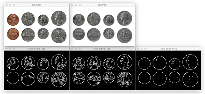
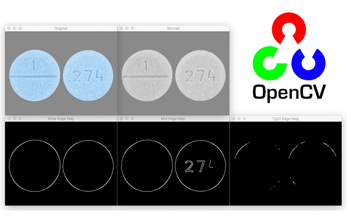
In the above figure, the top-left image is our input image of coins. We then blur the image slightly to help smooth details and aid in edge detection on the top-right.

The wide range, mid-range, and tight range edge maps are then displayed on the bottom, respectively.

Using a wide edge map captures the outlines of the coins, but also captures many of the edges of faces and symbols inside the coins.

The mid-range edge map also performs similarly.

Finally, the tight range edge map is able to capture just the outline of the coins while discarding the rest.

Let’s look at another example:

$ python opencv_canny.py --image images/clonazepam_1mg.png

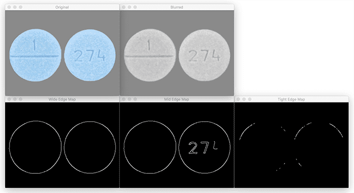
Unlike Figure 11, the Canny thresholds for Figure 12 give us nearly reversed results.

Using the wide range edge map, we are able to find the outlines of the pills.

The mid-range edge map also gives us the outlines of the pills, but also some of the digits imprinted on the pill.

Finally, the tight edge map does not help us at all — the outline of the pills is nearly completely lost.

How do we choose optimal Canny edge detection parameters?

As you can tell, depending on your input image you’ll need dramatically different hysteresis threshold values — and tuning these values can be a real pain. You might be wondering, is there a way to reliably tune these parameters without simply guessing, checking, and viewing the results?

The answer is yes!

We’ll be discussing that very technique in our next lesson.

Summary

In this lesson, we learned how to use image gradients, one of the most fundamental building blocks of computer vision and image processing, to create an edge detector.

Specifically, we focused on the Canny edge detector, the most well known and most used edge detector in the computer vision community.

From there, we examined the steps of the Canny edge detector including:

1. Smoothing
2. Computing image gradients
3. Applying non-maxima suppression
4. Utilizing hysteresis thresholding

We then took our knowledge of the Canny edge detector and used it to apply OpenCV’s cv2.Canny function to detect edges in images.

However, one of the biggest drawbacks of the Canny edge detector is tuning the upper and lower thresholds for the hysteresis step. If our threshold was too wide, we would get too many edges. And if our threshold was too tight, we would not detect many edges at all!

To aid us in parameter tuning you’ll learn how to apply automatic Canny edge detection in the next tutorial in this series.

To download the source code to this post (and be notified when future tutorials are published here on PyImageSearch), simply enter your email address in the form below!