Fire and smoke detection with Keras and Deep Learning

In this tutorial, you will learn how to detect fire and smoke using Computer Vision, OpenCV, and the Keras Deep Learning library.

Today’s tutorial is inspired by an email I received last week from PyImageSearch reader, Daniel.

Daniel writes:

Hey Adrian, I’m not sure if you’ve seen the news, but my home state of California has been absolutely ravaged by wildfires over the past few weeks.

My family lives in the Los Angeles area, not too far from the Getty fire. It’s hard not to be concerned about our home and our safety.

It’s a scary situation and it got me thinking:

Do you think computer vision could be used to detect wildfires? What about fires that start in people’s homes?

If you could write a tutorial on the topic I would appreciate it. I’d love to learn from it and do my part to help others.

The short answer is, yes, computer vision and deep learning can be used to detect wildfires:

• IoT/Edge devices equipped with cameras can be deployed strategically throughout hillsides, ridges, and high elevation areas, automatically monitoring for signs of smoke or fire.
• Drones and quadcopters can be flown above areas prone to wildfires, strategically scanning for smoke.
• Satellites can be used to take photos of large acreage areas while computer vision and deep learning algorithms process these images, looking for signs of smoke.

That’s all fine and good for wildfires — but what if you wanted to monitor your own home for smoke or fire?

The answer there is to augment existing sensors to aid in fire/smoke detection:

• Existing smoke detectors utilize photoelectric sensors and a light source to detect if the light source particles are being scattered (implying smoke is present).
• You could then distribute temperature sensors around the house to monitor the temperature of each room.
• Cameras could also be placed in areas where fires are likely to start (kitchen, garage, etc.).
• Each individual sensor could be used to trigger an alarm or you could relay the sensor information to a central hub that aggregates and analyzes the sensor data, computing a probability of a home fire.

Unfortunately, that’s all easier said than done.

While there are 100s of computer vision/deep learning practitioners around the world actively working on fire and smoke detection (including PyImageSearch Gurus member, David Bonn), it’s still an open-ended problem.

That said, today I’ll help you get your start in smoke and fire detection — by the end of this tutorial, you’ll have a deep learning model capable of detecting fire in images (I’ve even included my pre-trained model to get you up and running immediately).

To learn how to create your own fire and smoke detector with Computer Vision, Deep Learning, and Keras, just keep reading!

Fire and smoke detection with Keras and Deep Learning

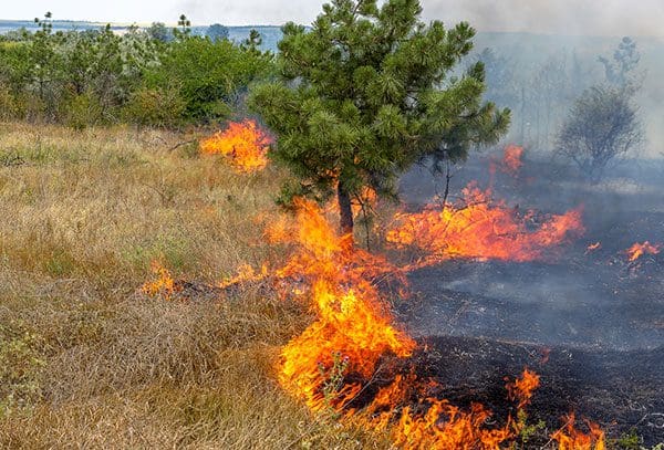
In the first part of this tutorial we’ll discuss the two datasets we’ll be using for fire and smoke detection.

From there we’ll review or directory structure for the project and then implement FireDetectionNet, the CNN architecture we’ll be using to detect fire and smoke in images/video.

Next, we’ll train our fire detection model and analyze the classification accuracy and results.

We’ll wrap up the tutorial by discussing some of the limitations and drawbacks of the approach, including how you can improve and extend the method.

Our fire and smoke dataset

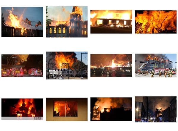
The dataset we’ll be using for fire and smoke examples was curated by PyImageSearch reader, Gautam Kumar.

Guatam gathered a total of 1,315 images by searching Google Images for queries related to the term “fire”, “smoke”, etc.

However, the original dataset has not been cleansed of extraneous, irrelevant images that are not related to fire and smoke (i.e., examples of famous buildings before a fire occurred).

Fellow PyImageSearch reader, David Bonn, took the time to manually go through the fire/smoke images and identify ones that should not be included.

Note: I took the list of extraneous images identified by David and then created a shell script to delete them from the dataset. The shell script can be found in the “Downloads” section of this tutorial.

The 8-scenes dataset

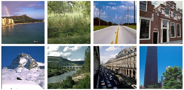
The dataset we’ll be using for Non-fire examples is called 8-scenes as it contains 2,688 image examples belonging to eight natural scene categories (all without fire):

1. Coast
2. Mountain
3. Forest
4. Open country
5. Street
6. Inside city
7. Tall buildings
8. Highways

The dataset was originally curated by Oliva and Torralba in their 2001 paper, Modeling the shape of the scene: a holistic representation of the spatial envelope.

The 8-scenes dataset is a natural complement to our fire/smoke dataset as it depicts natural scenes as they should look without fire or smoke present.

While this dataset has 8 unique classes, we will consider the dataset as a single Non-fire class when we combine it with Gautam’s Fire dataset.

Project structure

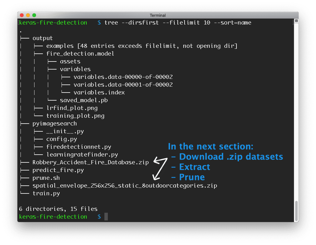
Go ahead and grab today’s .zip from the source code and pre-trained model using the “Downloads” section of this blog post.

From there you can unzip it on your machine and your project will look like Figure 4. There is an exception: neither dataset .zip (white arrows) will be present yet. We will download, extract, and prune the datasets in the next section.

Our output/ directory contains:

• Our serialized fire detection model. We will train the model today with Keras and deep learning.
• The Learning Rate Finder plot will be generated and inspected for the optimal learning rate prior to training.
• A training history plot will be generated upon completion of the training process.
• The examples/ subdirectory will be populated by predict_fire.py with sample images that will be annotated for demonstration and verification purposes.

Our pyimagesearch module holds:

• config.py : Our customizable configuration.
• FireDetectionNet : Our Keras Convolutional Neural Network class designed specifically for detecting fire and smoke.
• LearningRateFinder : A Keras class for assisting in the process of finding the optimal learning rate for deep learning training.

The root of the project contains three scripts:

• prune.sh : A simple bash script that removes irrelevant images from Gautam’s fire dataset.
• train.py : Our Keras deep learning training script. This script has two modes of operation: (1) Learning Rate Finder mode,and (2) training mode.
• predict_fire.py : A quick and dirty script which samples images from our dataset, generating annotated Fire/Non-fire images for verification.

Let’s move on to preparing our Fire/Non-fire dataset in the next section.

Preparing our Fire and Non-fire combined dataset

Preparing our Fire and Non-fire dataset involves a four-step process:

1. Step #1: Ensure you followed the instructions in the previous section to grab and unzip today’s files from the “Downloads” section.
2. Step #2: Download and extract the fire/smoke dataset into the project.
3. Step #3: Prune the fire/smoke dataset for extraneous, irrelevant files.
4. Step #4: Download and extract the 8-scenes dataset into the project.

The result of Steps #2-4 will be a dataset consisting of two classes:

• Fire
• Non-fire

Combining datasets is a tactic I often use. It saves valuable time and often leads to a great model.

Let’s begin putting our combined dataset together.

Step #2: Download and extract the fire/smoke dataset into the project.

Download the fire/smoke dataset using this link. Store the .zip in the keras-fire-detection/ project directory that you extracted in the last section.

Once downloaded, unzip the dataset:

$ unzip Robbery_Accident_Fire_Database2.zip

Step #3: Prune the dataset for extraneous, irrelevant files.

Execute the prune.sh script to delete the extraneous, irrelevant files from the fire dataset:

$ sh prune.sh

At this point, we have Fire data. Now we need Non-fire data for our two-class problem.

Step #4: Download and extract the 8-scenes dataset into the project.

Download the 8-scenes dataset using this link. Store the .zip in the keras-fire-detection/ project directory alongside the Fire dataset.

Once downloaded, navigate to the project folder and unarchive the dataset:

$ unzip spatial_envelope_256x256_static_8outdoorcategories.zip

Review Project + Dataset Structure

At this point, it is time to inspect our directory structure once more. Yours should be identical to mine:

$ tree --dirsfirst --filelimit 10
.
├── Robbery_Accident_Fire_Database2
│   ├── Accident [887 entries]
│   ├── Fire [1315 entries]
│   ├── Robbery [2073 entries]
│   └── readme.txt
├── spatial_envelope_256x256_static_8outdoorcategories [2689 entries]
├── output
│   ├── examples [48 entries]
│   ├── fire_detection.model
│   │   ├── assets
│   │   ├── variables
│   │   │   ├── variables.data-00000-of-00002
│   │   │   ├── variables.data-00001-of-00002
│   │   │   └── variables.index
│   │   └── saved_model.pb
│   ├── lrfind_plot.png
│   └── training_plot.png
├── pyimagesearch
│   ├── __init__.py
│   ├── config.py
│   ├── firedetectionnet.py
│   └── learningratefinder.py
├── Robbery_Accident_Fire_Database.zip
├── spatial_envelope_256x256_static_8outdoorcategories.zip
├── prune.sh
├── train.py
└── predict_fire.py

11 directories, 16 files

Ensure your dataset is pruned (i.e. the Fire/ directory should have exactly 1,315 entries and not the previous 1,405 entries).

Our configuration file

This project will span multiple Python files that will need to be executed, so let’s store all important variables in a single config.py file.

Open up config.py now and insert the following code:

# import the necessary packages
import os

# initialize the path to the fire and non-fire dataset directories
FIRE_PATH = os.path.sep.join(["Robbery_Accident_Fire_Database2",
	"Fire"])
NON_FIRE_PATH = "spatial_envelope_256x256_static_8outdoorcategories"

# initialize the class labels in the dataset
CLASSES = ["Non-Fire", "Fire"]

We’ll use the os module for combining paths (Line 2).

Lines 5-7 contain paths to our (1) Fire images, and (2) Non-fire images.

Line 10 is a list of our two class names.

Let’s set a handful of training parameters:

# define the size of the training and testing split
TRAIN_SPLIT = 0.75
TEST_SPLIT = 0.25

# define the initial learning rate, batch size, and number of epochs
INIT_LR = 1e-2
BATCH_SIZE = 64
NUM_EPOCHS = 50

Lines 13 and 14 define the size of our training and testing dataset splits.

Lines 17-19 contain three hyperparameters — the initial learning rate, batch size, and number of epochs to train for.

From here, we’ll define a few paths:

# set the path to the serialized model after training
MODEL_PATH = os.path.sep.join(["output", "fire_detection.model"])

# define the path to the output learning rate finder plot and
# training history plot
LRFIND_PLOT_PATH = os.path.sep.join(["output", "lrfind_plot.png"])
TRAINING_PLOT_PATH = os.path.sep.join(["output", "training_plot.png"])

Lines 22-27 include paths to:

• Our yet-to-be-trained serialized fire detection model.
• The Learning Rate Finder plot which we will analyze to set our initial learning rate.
• A training accuracy/loss history plot.

To wrap up our config we’ll define settings for prediction spot-checking:

# define the path to the output directory that will store our final
# output with labels/annotations along with the number of images to
# sample
OUTPUT_IMAGE_PATH = os.path.sep.join(["output", "examples"])
SAMPLE_SIZE = 50

Our prediction script will sample and annotate images using our model.

Lines 32 and 33 include the path to output directory where we’ll store output classification results and the number of images to sample.

Implementing our fire detection Convolutional Neural Network

In this section we’ll implement FireDetectionNet, a Convolutional Neural Network used to detect smoke and fire in images.

This network utilizes depthwise separable convolution rather than standard convolution as depthwise separable convolution:

• Is more efficient, as Edge/IoT devices will have limited CPU and power draw.
• Requires less memory, as again, Edge/IoT devices have limited RAM.
• Requires less computation, as we have limited CPU horsepower.
• Can perform better than standard convolution in some cases, which can lead to a better fire/smoke detector.

Let’s get started implementing FireDetectioNet now — open up the firedetectionnet.py file now and insert the following code:

# import the necessary packages
from tensorflow.keras.models import Sequential
from tensorflow.keras.layers import BatchNormalization
from tensorflow.keras.layers import SeparableConv2D
from tensorflow.keras.layers import MaxPooling2D
from tensorflow.keras.layers import Activation
from tensorflow.keras.layers import Flatten
from tensorflow.keras.layers import Dropout
from tensorflow.keras.layers import Dense

class FireDetectionNet:
	@staticmethod
	def build(width, height, depth, classes):
		# initialize the model along with the input shape to be
		# "channels last" and the channels dimension itself
		model = Sequential()
		inputShape = (height, width, depth)
		chanDim = -1

Our TensorFlow 2.0 Keras imports span from Lines 2-9. We will use Keras’ Sequential API to build our fire detection CNN.

Line 11 defines our FireDetectionNet class. We begin by defining the build method on Line 13.

The build method accepts parameters including dimensions of our images (width , height , depth ) as well as the number of classes we will be training our model to recognize (i.e. this parameter affects the softmax classifier head shape).

We then initialize the model and inputShape (Lines 16-18).

From here we’ll define our first set of CONV => RELU => POOL layers:

		# CONV => RELU => POOL
		model.add(SeparableConv2D(16, (7, 7), padding="same",
			input_shape=inputShape))
		model.add(Activation("relu"))
		model.add(BatchNormalization(axis=chanDim))
		model.add(MaxPooling2D(pool_size=(2, 2)))

These layers use a larger kernel size to both (1) reduce the input volume spatial dimensions faster, and (2) detect larger color blobs that contain fire.

We’ll then define more CONV => RELU => POOL layer sets:

		# CONV => RELU => POOL
		model.add(SeparableConv2D(32, (3, 3), padding="same"))
		model.add(Activation("relu"))
		model.add(BatchNormalization(axis=chanDim))
		model.add(MaxPooling2D(pool_size=(2, 2)))

		# (CONV => RELU) * 2 => POOL
		model.add(SeparableConv2D(64, (3, 3), padding="same"))
		model.add(Activation("relu"))
		model.add(BatchNormalization(axis=chanDim))
		model.add(SeparableConv2D(64, (3, 3), padding="same"))
		model.add(Activation("relu"))
		model.add(BatchNormalization(axis=chanDim))
		model.add(MaxPooling2D(pool_size=(2, 2)))

Lines 34-40 allow our model to learn richer features by stacking two sets of CONV => RELU before applying a POOL .

From here we’ll create our fully-connected head of the network:

		# first set of FC => RELU layers
		model.add(Flatten())
		model.add(Dense(128))
		model.add(Activation("relu"))
		model.add(BatchNormalization())
		model.add(Dropout(0.5))

		# second set of FC => RELU layers
		model.add(Dense(128))
		model.add(Activation("relu"))
		model.add(BatchNormalization())
		model.add(Dropout(0.5))

		# softmax classifier
		model.add(Dense(classes))
		model.add(Activation("softmax"))

		# return the constructed network architecture
		return model

Lines 43-53 add two sets of FC => RELU layers.

Lines 56 and 57 append our Softmax classifier prior to Line 60 returning the model .

Creating our training script

Our training script will be responsible for:

1. Loading our Fire and Non-fire combined dataset from disk.
2. Instantiating our FireDetectionNet architecture.
3. Finding our optimal learning rate by using our LearningRateFinder class.
4. Taking the optimal learning rate and training our network for the full set of epochs.

Let’s get started!

Open up the train.py file in your directory structure and insert the following code:

# set the matplotlib backend so figures can be saved in the background
import matplotlib
matplotlib.use("Agg")

# import the necessary packages
from tensorflow.keras.preprocessing.image import ImageDataGenerator
from tensorflow.keras.optimizers import SGD
from tensorflow.keras.utils import to_categorical
from sklearn.model_selection import train_test_split
from sklearn.metrics import classification_report
from pyimagesearch.learningratefinder import LearningRateFinder
from pyimagesearch.firedetectionnet import FireDetectionNet
from pyimagesearch import config
from imutils import paths
import matplotlib.pyplot as plt
import numpy as np
import argparse
import cv2
import sys

Lines 1-19 handle our imports:

• matplotlib : For generating plots with Python. Line 3 sets the backend so we can save our plots as image files.
• tensorflow.keras : Our TensorFlow 2.0 imports including data augmentation, stochastic gradient descent optimizer, and one-hot label encoder.
• sklearn : Two imports for dataset splitting and classification reporting.
• LearningRateFinder : A class we will use for finding an optimal learning rate prior to training. When we operate our script in this mode, it will generate a plot for us to (1) manually inspect and (2) insert the optimal learning rate into our configuration file.
• FireDetectionNet : The fire/smoke Convolutional Neural Network (CNN) that we built in the previous section.
• config : Our configuration file of settings for this training script (it also contains settings for our prediction script).
• paths : Contains functions from my imutils package to list images in a directory tree.
• argparse : For parsing command line argument flags.
• cv2 : OpenCV is used for loading and preprocessing images.

Now that we’ve imported packages, let’s define a reusable function to load our dataset:

def load_dataset(datasetPath):
	# grab the paths to all images in our dataset directory, then
	# initialize our lists of images
	imagePaths = list(paths.list_images(datasetPath))
	data = []

	# loop over the image paths
	for imagePath in imagePaths:
		# load the image and resize it to be a fixed 128x128 pixels,
		# ignoring aspect ratio
		image = cv2.imread(imagePath)
		image = cv2.resize(image, (128, 128))

		# add the image to the data lists
		data.append(image)

	# return the data list as a NumPy array
	return np.array(data, dtype="float32")

Our load_dataset helper function assists with loading, preprocessing, and preparing both the Fire and Non-fire datasets.

Line 21 defines the function which accepts a path to the dataset.

Line 24 grabs all image paths in the dataset.

Lines 28-35 loop over the imagePaths . Images are loaded, resized to 128×128 dimensions, and added to the data list.

Line 38 returns the data in NumPy array format.

We’ll now parse a single command line argument:

# construct the argument parser and parse the arguments
ap = argparse.ArgumentParser()
ap.add_argument("-f", "--lr-find", type=int, default=0,
	help="whether or not to find optimal learning rate")
args = vars(ap.parse_args())

The --lr-find flag sets the mode for our script. If the flag is set to 1 , then we’ll be in our learning rate finder mode, generating a learning rate plot for us to inspect. Otherwise, our script will operate in training mode and train the network for the full set of epochs (i.e. when the --lr-find flag is not present).

Let’s go ahead and load our data now:

# load the fire and non-fire images
print("[INFO] loading data...")
fireData = load_dataset(config.FIRE_PATH)
nonFireData = load_dataset(config.NON_FIRE_PATH)

# construct the class labels for the data
fireLabels = np.ones((fireData.shape[0],))
nonFireLabels = np.zeros((nonFireData.shape[0],))

# stack the fire data with the non-fire data, then scale the data
# to the range [0, 1]
data = np.vstack([fireData, nonFireData])
labels = np.hstack([fireLabels, nonFireLabels])
data /= 255

Lines 48 and 49 load and resize the Fire and Non-fire images.

Lines 52 and 53 construct labels for both classes (1 for Fire and 0 for Non-fire).

Subsequently, we stack the data and labels into a single NumPy array (i.e. combine the datasets) via Lines 57 and 58.

Line 59 scales pixel intensities to the range [0, 1].

We have three more steps to prepare our data:

# perform one-hot encoding on the labels and account for skew in the
# labeled data
labels = to_categorical(labels, num_classes=2)
classTotals = labels.sum(axis=0)
classWeight = classTotals.max() / classTotals

# construct the training and testing split
(trainX, testX, trainY, testY) = train_test_split(data, labels,
	test_size=config.TEST_SPLIT, random_state=42)

First, we perform one-hot encoding on our labels (Line 63).

Then, we account for skew in our dataset (Lines 64 and 65). To do so, we compute the classWeight to weight Fire images more than Non-fire images during the gradient update (as we have over 2x more Fire images than Non-fire images).

Lines 68 and 69 construct training and testing splits based on our config (in my config I have the split set to 75% training/25% testing).

Next, we’ll initialize data augmentation and compile our FireDetectionNet model:

# initialize the training data augmentation object
aug = ImageDataGenerator(
	rotation_range=30,
	zoom_range=0.15,
	width_shift_range=0.2,
	height_shift_range=0.2,
	shear_range=0.15,
	horizontal_flip=True,
	fill_mode="nearest")

# initialize the optimizer and model
print("[INFO] compiling model...")
opt = SGD(lr=config.INIT_LR, momentum=0.9,
	decay=config.INIT_LR / config.NUM_EPOCHS)
model = FireDetectionNet.build(width=128, height=128, depth=3,
	classes=2)
model.compile(loss="binary_crossentropy", optimizer=opt,
	metrics=["accuracy"])

Lines 74-79 instantiate our data augmentation object.

We then build and compile our FireDetectionNet model (Lines 83-88). Note that our initial learning rate and decay is set as we initialize our SGD optimizer.

Let’s handle our Learning Rate Finder mode:

# check to see if we are attempting to find an optimal learning rate
# before training for the full number of epochs
if args["lr_find"] > 0:
	# initialize the learning rate finder and then train with learning
	# rates ranging from 1e-10 to 1e+1
	print("[INFO] finding learning rate...")
	lrf = LearningRateFinder(model)
	lrf.find(
		aug.flow(trainX, trainY, batch_size=config.BATCH_SIZE),
		1e-10, 1e+1,
		stepsPerEpoch=np.ceil((trainX.shape[0] / float(config.BATCH_SIZE))),
		epochs=20,
		batchSize=config.BATCH_SIZE,
		classWeight=classWeight)

	# plot the loss for the various learning rates and save the
	# resulting plot to disk
	lrf.plot_loss()
	plt.savefig(config.LRFIND_PLOT_PATH)

	# gracefully exit the script so we can adjust our learning rates
	# in the config and then train the network for our full set of
	# epochs
	print("[INFO] learning rate finder complete")
	print("[INFO] examine plot and adjust learning rates before training")
	sys.exit(0)

Line 92 checks to see if we should attempt to find optimal learning rates. Assuming so, we:

• Initialize LearningRateFinder (Line 96).
• Start training with a 1e-10 learning rate and exponentially increase it until we hit 1e+1 (Lines 97-103).
• Plot the loss vs. learning rate and save the resulting figure (Lines 107 and 108).
• Gracefully exit the script after printing a couple of messages to the user (Lines 115).

After this code executes we now need to:

1. Step #1: Manually inspect the generated learning rate plot.
2. Step #2: Update config.py with our INIT_LR (i.e., the optimal learning rate we determined by analyzing the plot).
3. Step #3: Train the network on our full dataset.

Assuming we have completed Step #1 and Step #2, now let’s handle the Step #3 where our initial learning rate has been determined and updated in the config. In this case, it is time to handle training mode in our script:

# train the network
print("[INFO] training network...")
H = model.fit_generator(
	aug.flow(trainX, trainY, batch_size=config.BATCH_SIZE),
	validation_data=(testX, testY),
	steps_per_epoch=trainX.shape[0] // config.BATCH_SIZE,
	epochs=config.NUM_EPOCHS,
	class_weight=classWeight,
	verbose=1)

Lines 119-125 train our fire detection model using data augmentation and our skewed dataset class weighting. Be sure to review my .fit_generator tutorial.

Finally, we’ll evaluate the model, serialize it to disk, and plot the training history:

# evaluate the network and show a classification report
print("[INFO] evaluating network...")
predictions = model.predict(testX, batch_size=config.BATCH_SIZE)
print(classification_report(testY.argmax(axis=1),
	predictions.argmax(axis=1), target_names=config.CLASSES))

# serialize the model to disk
print("[INFO] serializing network to '{}'...".format(config.MODEL_PATH))
model.save(config.MODEL_PATH)

# construct a plot that plots and saves the training history
N = np.arange(0, config.NUM_EPOCHS)
plt.style.use("ggplot")
plt.figure()
plt.plot(N, H.history["loss"], label="train_loss")
plt.plot(N, H.history["val_loss"], label="val_loss")
plt.plot(N, H.history["accuracy"], label="train_acc")
plt.plot(N, H.history["val_accuracy"], label="val_acc")
plt.title("Training Loss and Accuracy")
plt.xlabel("Epoch #")
plt.ylabel("Loss/Accuracy")
plt.legend(loc="lower left")
plt.savefig(config.TRAINING_PLOT_PATH)

Lines 129-131 make predictions on test data and print a classification report in our terminal.

Line 135 serializes the model and saves it to disk. We’ll recall the model in our prediction script.

Lines 138-149 generate a historical plot of accuracy/loss curves during training. We will inspect this plot for overfitting or underfitting.

Training the fire detection model with Keras

Training our fire detection model is broken down into three steps:

1. Step #1: Run the train.py script with the --lr-find command line argument to find our optimal learning rate.
2. Step #2: Update Line 17 of our configuration file (config.py ) to set our INIT_LR value as the optimal learning rate.
3. Step #3: Execute the train.py script again, but this time let it train for the full set of epochs.

Start by using the “Downloads” section of this tutorial to download the source code to this tutorial.

From there you can perform Step #1 by executing the following command:

$ python train.py --lr-find 1
[INFO] loading data...
[INFO] finding learning rate...
Epoch 1/20
47/47 [==============================] - 10s 221ms/step - loss: 1.2949 - accuracy: 0.4923
Epoch 2/20
47/47 [==============================] - 11s 228ms/step - loss: 1.3315 - accuracy: 0.4897
Epoch 3/20
47/47 [==============================] - 10s 218ms/step - loss: 1.3409 - accuracy: 0.4860
Epoch 4/20
47/47 [==============================] - 10s 215ms/step - loss: 1.3973 - accuracy: 0.4770
Epoch 5/20
47/47 [==============================] - 10s 219ms/step - loss: 1.3170 - accuracy: 0.4957
...
Epoch 15/20
47/47 [==============================] - 10s 216ms/step - loss: 0.5097 - accuracy: 0.7728
Epoch 16/20
47/47 [==============================] - 10s 217ms/step - loss: 0.5507 - accuracy: 0.7345
Epoch 17/20
47/47 [==============================] - 10s 220ms/step - loss: 0.7554 - accuracy: 0.7089
Epoch 18/20
47/47 [==============================] - 10s 220ms/step - loss: 1.1833 - accuracy: 0.6606
Epoch 19/20
37/47 [======================>.......] - ETA: 2s - loss: 3.1446 - accuracy: 0.6338
[INFO] learning rate finder complete
[INFO] examine plot and adjust learning rates before training

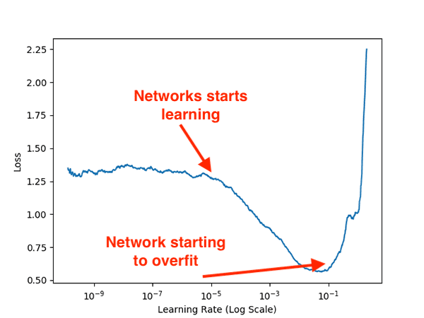
Examining Figure 6 above you can see that our network is able to gain traction and start to learn around 1e-5 .

The lowest loss can be found between 1e-2 and 1e-1; however, at 1e-1 we can see loss starting to increase sharply, implying that the learning rate is too large and the network is overfitting.

To be safe we should use an initial learning rate of 1e-2.

Let’s now move on to Step #2.

Open up config.py and scroll to Lines 16-19 where we set our training hyperparameters:

# define the initial learning rate, batch size, and number of epochs
INIT_LR = 1e-2
BATCH_SIZE = 64
NUM_EPOCHS = 50

Here we see our initial learning rate (INIT_LR) value — we need to set this value to 1e-2 (as our code indicates).

The final step (Step #3) is to train FireDetectionNet for the full set of NUM_EPOCHS:

$ python train.py
[INFO] loading data...
[INFO] compiling model...
[INFO] training network...
Epoch 1/50
46/46 [==============================] - 11s 233ms/step - loss: 0.6813 - accuracy: 0.6974 - val_loss: 0.6583 - val_accuracy: 0.6464
Epoch 2/50
46/46 [==============================] - 11s 232ms/step - loss: 0.4886 - accuracy: 0.7631 - val_loss: 0.7774 - val_accuracy: 0.6464
Epoch 3/50
46/46 [==============================] - 10s 224ms/step - loss: 0.4414 - accuracy: 0.7845 - val_loss: 0.9470 - val_accuracy: 0.6464
Epoch 4/50
46/46 [==============================] - 10s 222ms/step - loss: 0.4193 - accuracy: 0.7917 - val_loss: 1.0790 - val_accuracy: 0.6464
Epoch 5/50
46/46 [==============================] - 10s 224ms/step - loss: 0.4015 - accuracy: 0.8070 - val_loss: 1.2034 - val_accuracy: 0.6464
...
Epoch 46/50
46/46 [==============================] - 10s 222ms/step - loss: 0.1935 - accuracy: 0.9275 - val_loss: 0.2985 - val_accuracy: 0.8781
Epoch 47/50
46/46 [==============================] - 10s 221ms/step - loss: 0.1812 - accuracy: 0.9244 - val_loss: 0.2325 - val_accuracy: 0.9031
Epoch 48/50
46/46 [==============================] - 10s 226ms/step - loss: 0.1857 - accuracy: 0.9241 - val_loss: 0.2788 - val_accuracy: 0.8911
Epoch 49/50
46/46 [==============================] - 11s 229ms/step - loss: 0.2065 - accuracy: 0.9129 - val_loss: 0.2177 - val_accuracy: 0.9121
Epoch 50/50
46/46 [==============================] - 63s 1s/step - loss: 0.1842 - accuracy: 0.9316 - val_loss: 0.2376 - val_accuracy: 0.9111
[INFO] evaluating network...
              precision    recall  f1-score   support

    Non-Fire       0.96      0.90      0.93       647
        Fire       0.83      0.94      0.88       354

    accuracy                           0.91      1001
   macro avg       0.90      0.92      0.91      1001
weighted avg       0.92      0.91      0.91      1001

[INFO] serializing network to 'output/fire_detection.model'...

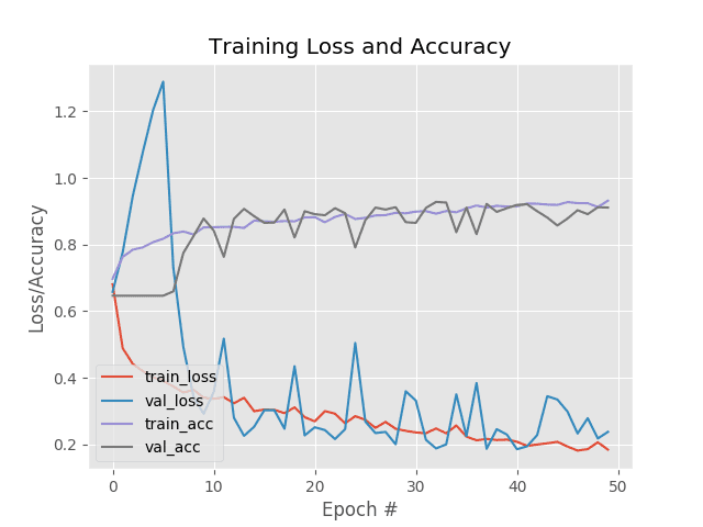
Learning is a bit volatile here but you can see that we are obtaining 92% accuracy.

Making predictions on fire/non-fire images

Given our trained fire detection model, let’s now learn how to:

1. Load the trained model from disk.
2. Sample random images from our dataset.
3. Classify each input image using our model.

Open up predict_fire.py and insert the following code:

# import the necessary packages
from tensorflow.keras.models import load_model
from pyimagesearch import config
from imutils import paths
import numpy as np
import imutils
import random
import cv2
import os

# load the trained model from disk
print("[INFO] loading model...")
model = load_model(config.MODEL_PATH)

Lines 2-9 handle our imports, namely load_model , so that we can load our serialized TensorFlow/Keras model from disk.

Let’s grab 25 random images from our combined dataset:

# grab the paths to the fire and non-fire images, respectively
print("[INFO] predicting...")
firePaths = list(paths.list_images(config.FIRE_PATH))
nonFirePaths = list(paths.list_images(config.NON_FIRE_PATH))

# combine the two image path lists, randomly shuffle them, and sample
# them
imagePaths = firePaths + nonFirePaths
random.shuffle(imagePaths)
imagePaths = imagePaths[:config.SAMPLE_SIZE]

Lines 17 and 18 grab image paths from our combined dataset while Lines 22-24 sample 25 random image paths.

From here, we’ll loop over each of the individual image paths and perform fire detection inference:

# loop over the sampled image paths
for (i, imagePath) in enumerate(imagePaths):
	# load the image and clone it
	image = cv2.imread(imagePath)
	output = image.copy()

	# resize the input image to be a fixed 128x128 pixels, ignoring
	# aspect ratio
	image = cv2.resize(image, (128, 128))
	image = image.astype("float32") / 255.0
		
	# make predictions on the image
	preds = model.predict(np.expand_dims(image, axis=0))[0]
	j = np.argmax(preds)
	label = config.CLASSES[j]

	# draw the activity on the output frame
	text = label if label == "Non-Fire" else "WARNING! Fire!"
	output = imutils.resize(output, width=500)
	cv2.putText(output, text, (35, 50), cv2.FONT_HERSHEY_SIMPLEX,
		1.25, (0, 255, 0), 5)

	# write the output image to disk	 
	filename = "{}.png".format(i)
	p = os.path.sep.join([config.OUTPUT_IMAGE_PATH, filename])
	cv2.imwrite(p, output)

Line 27 begins a loop over our sampled image paths:

• We load and preprocess the image just as in training (Lines 29-35).
• Make predictions and grab the highest probability label (Lines 38-40).
• Annotate the label in the top corner of the image (Lines 43-46).
• Save the output image to disk (Lines 49-51).

Fire detection results

To see our fire detector in action make sure you use the “Downloads” section of this tutorial to download the source code and pre-trained model.

From there you can execute the following command:

$ python predict_fire.py
[INFO] loading model...
[INFO] predicting...

I’ve included a set sample of results in Figure 8 — notice how our model was able to correctly predict “fire” and “non-fire” in each of them.

Limitations and drawbacks

Our results are not perfect, however. Here are a few examples of incorrect classifications:

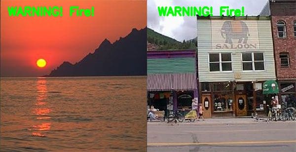
The image on the left in particular is troubling — a sunset will cast shades of reds and oranges across the sky, creating an “inferno” like effect. It appears that in those situations our fire detection model will struggle considerably.

So, why are these incorrect classifications coming from?

The answer lies in the dataset itself.

To start, we only worked with raw image data.

Smoke and fire can be better detected with video as fires start off as a smolder, slowly build to a critical point, and then erupt into massive flames. Such a pattern is better detected in video streams rather than images.

Secondly, our datasets are quite small.

Combining the two datasets we only had a total of 4,003 images. Fire and smoke datasets are hard to come by, making it extremely challenging to create high accuracy models.

Finally, our datasets are not necessarily representative of the problem.

Many of the example images in our fire/smoke dataset contained examples of professional photos captured by news reports. Fires don’t look like that in the wild.

In order to improve our fire and smoke detection model, we need better data.

Future efforts in fire/smoke detection research should focus less on the actual deep learning architectures/training methods and more on the actual dataset gathering and curation process, ensuring the dataset better represents how fires start, smolder, and spread in natural scene images.

Summary

In this tutorial, you learned how to create a smoke and fire detector using Computer Vision, Deep Learning, and the Keras library.

To build our smoke and fire detector we utilized two datasets:

• A dataset of fire/smoke examples (1,315 images), curated by PyImageSearch readers Gautam Kumar.
• A dataset of non-fire/non-smoke examples (2,688 images) containing examples of 8 natural outdoor scenes (forests, coastlines, mountains, open country, etc.). This dataset was originally put together by Oliva and Torralba for their 2001 paper, Modeling the shape of the scene: a holistic representation of the spatial envelope.

We then designed a FireDetectionNet — a Convolutional Neural Network for smoke and fire detection. This network was trained on our two datasets. Once our network was trained we evaluated it on our testing set and found that it obtained 92% accuracy.

However, there are a number of limitations and drawbacks to this approach:

• First, we only worked with image data. Smoke and fire can be better detected with video as fires start off as a smolder, slowly build to a critical point, and then erupt into massive flames.
• Secondly, our datasets are small. Combining the two datasets we only had a total of 4,003 images. Fire and smoke datasets are hard to come by, making it extremely challenging to create high accuracy models.

Building on the previous point, our datasets are not necessarily representative of the problem. Many of the example images in our fire/smoke dataset are of professional photos captured by news reports. Fires don’t look like that in the wild.

The point is this:

Fire and smoke detection is a solvable problem…but we need better datasets.

Luckily, PyImageSearch Gurus member David Bonn is actively working on this problem and discussing it in the PyImageSearch Gurus Community forums. If you’re interested in learning more about his project, be sure to connect with him.

I hope you enjoyed this tutorial!

To download the source code to this post (and be notified when future tutorials are published here on PyImageSearch), just enter your email address in the form below.