Fashion MNIST with Keras and Deep Learning

In this tutorial, you will learn how to train a simple Convolutional Neural Network (CNN) with Keras on the Fashion MNIST dataset, enabling you to classify fashion images and categories.

The Fashion MNIST dataset is meant to be a (slightly more challenging) drop-in replacement for the (less challenging) MNIST dataset.

Similar to the MNIST digit dataset, the Fashion MNIST dataset includes:

• 60,000 training examples
• 10,000 testing examples
• 10 classes
• 28×28 grayscale/single channel images

The ten fashion class labels include:

1. T-shirt/top
2. Trouser/pants
3. Pullover shirt
4. Dress
5. Coat
6. Sandal
7. Shirt
8. Sneaker
9. Bag
10. Ankle boot

Throughout this tutorial, you will learn how to train a simple Convolutional Neural Network (CNN) with Keras on the Fashion MNIST dataset, giving you not only hands-on experience working with the Keras library but also your first taste of clothing/fashion classification.

To learn how to train a Keras CNN on the Fashion MNIST dataset, just keep reading!

Fashion MNIST with Keras and Deep Learning

2020-06-11 Update: This blog post is now TensorFlow 2+ compatible!

In the first part of this tutorial, we will review the Fashion MNIST dataset, including how to download it to your system.

From there we’ll define a simple CNN network using the Keras deep learning library.

Finally, we’ll train our CNN model on the Fashion MNIST dataset, evaluate it, and review the results.

Let’s go ahead and get started!

The Fashion MNIST dataset

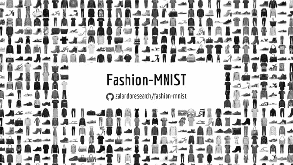
The Fashion MNIST dataset was created by e-commerce company, Zalando.

As they note on their official GitHub repo for the Fashion MNIST dataset, there are a few problems with the standard MNIST digit recognition dataset:

1. It’s far too easy for standard machine learning algorithms to obtain 97%+ accuracy.
2. It’s even easier for deep learning models to achieve 99%+ accuracy.
3. The dataset is overused.
4. MNIST cannot represent modern computer vision tasks.

Zalando, therefore, created the Fashion MNIST dataset as a drop-in replacement for MNIST.

The Fashion MNIST dataset is identical to the MNIST dataset in terms of training set size, testing set size, number of class labels, and image dimensions:

• 60,000 training examples
• 10,000 testing examples
• 10 classes
• 28×28 grayscale images

If you’ve ever trained a network on the MNIST digit dataset then you can essentially change one or two lines of code and train the same network on the Fashion MNIST dataset!

How to install TensorFlow/Keras

To configure your system for this tutorial, I first recommend following either of these tutorials:

• How to install TensorFlow 2.0 on Ubuntu
• How to install TensorFlow 2.0 on macOS

Either tutorial will help you configure you system with all the necessary software for this blog post in a convenient Python virtual environment.

Please note that PyImageSearch does not recommend or support Windows for CV/DL projects.

Obtaining the Fashion MNIST dataset

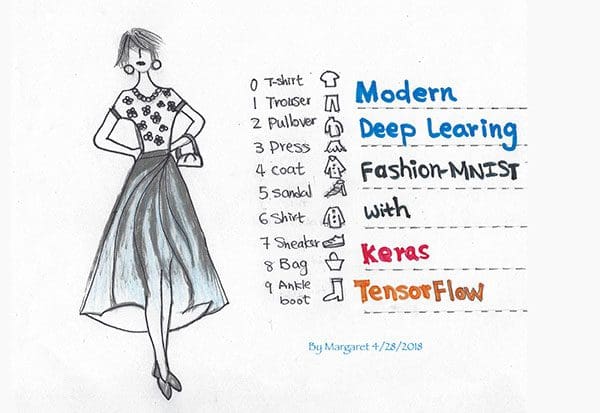
There are two ways to obtain the Fashion MNIST dataset.

If you are using the TensorFlow/Keras deep learning library, the Fashion MNIST dataset is actually built directly into the datasets module:

from tensorflow.keras.datasets import fashion_mnist
((trainX, trainY), (testX, testY)) = fashion_mnist.load_data()

Otherwise, if you are using another deep learning library you can download it directory from the the official Fashion MNIST GitHub repo.

A big thanks to Margaret Maynard-Reid for putting together the awesome illustration in Figure 2.

Project structure

To follow along, be sure to grab the “Downloads” for today’s blog post.

Once you’ve unzipped the files, your directory structure will look like this:

$ tree --dirsfirst
.
├── pyimagesearch
│   ├── __init__.py
│   └── minivggnet.py
├── fashion_mnist.py
└── plot.png

1 directory, 4 files

Our project today is rather straightforward — we’re reviewing two Python files:

• pyimagesearch/minivggnet.py : Contains a simple CNN based on VGGNet.
• fashion_mnist.py : Our training script for Fashion MNIST classification with Keras and deep learning. This script will load the data (remember, it is built into Keras), and train our MiniVGGNet model. A classification report and montage will be generated upon training completion.

Defining a simple Convolutional Neural Network (CNN)

Today we’ll be defining a very simple Convolutional Neural Network to train on the Fashion MNIST dataset.

We’ll call this CNN “MiniVGGNet” since:

• The model is inspired by its bigger brother, VGGNet
• The model has VGGNet characteristics, including:
  • Only using 3×3 CONV filters
  • Stacking multiple CONV layers before applying a max-pooling operation

We’ve used the MiniVGGNet model before a handful of times on the PyImageSearch blog but we’ll briefly review it here today as a matter of completeness.

Open up a new file, name it minivggnet.py, and insert the following code:

# import the necessary packages
from tensorflow.keras.models import Sequential
from tensorflow.keras.layers import BatchNormalization
from tensorflow.keras.layers import Conv2D
from tensorflow.keras.layers import MaxPooling2D
from tensorflow.keras.layers import Activation
from tensorflow.keras.layers import Flatten
from tensorflow.keras.layers import Dropout
from tensorflow.keras.layers import Dense
from tensorflow.keras import backend as K

class MiniVGGNet:
	@staticmethod
	def build(width, height, depth, classes):
		# initialize the model along with the input shape to be
		# "channels last" and the channels dimension itself
		model = Sequential()
		inputShape = (height, width, depth)
		chanDim = -1

		# if we are using "channels first", update the input shape
		# and channels dimension
		if K.image_data_format() == "channels_first":
			inputShape = (depth, height, width)
			chanDim = 1

Our Keras imports are listed on Lines 2-10. Our Convolutional Neural Network model is relatively simple, but we will be taking advantage of batch normalization and dropout which are two methods I nearly always recommend. For further reading please take a look at Deep Learning for Computer Vision with Python.

Our MiniVGGNet class and its build method are defined on Lines 12-14. The build function accepts four parameters:

• width : Image width in pixels.
• height : Image height in pixels.
• depth : Number of channels. Typically for color this value is 3 and for grayscale it is 1 (the Fashion MNIST dataset is grayscale).
• classes : The number of types of fashion articles we can recognize. The number of classes affects the final fully-connected output layer. For the Fashion MNIST dataset there are a total of 10 classes.

Our model is initialized on Line 17 using the Sequential API.

From there, our inputShape is defined (Line 18). We’re going to use "channels_last" ordering since our backend is TensorFlow, but in case you’re using a different backend, Lines 23-25 will accommodate.

Now let’s add our layers to the CNN:

		# first CONV => RELU => CONV => RELU => POOL layer set
		model.add(Conv2D(32, (3, 3), padding="same",
			input_shape=inputShape))
		model.add(Activation("relu"))
		model.add(BatchNormalization(axis=chanDim))
		model.add(Conv2D(32, (3, 3), padding="same"))
		model.add(Activation("relu"))
		model.add(BatchNormalization(axis=chanDim))
		model.add(MaxPooling2D(pool_size=(2, 2)))
		model.add(Dropout(0.25))

		# second CONV => RELU => CONV => RELU => POOL layer set
		model.add(Conv2D(64, (3, 3), padding="same"))
		model.add(Activation("relu"))
		model.add(BatchNormalization(axis=chanDim))
		model.add(Conv2D(64, (3, 3), padding="same"))
		model.add(Activation("relu"))
		model.add(BatchNormalization(axis=chanDim))
		model.add(MaxPooling2D(pool_size=(2, 2)))
		model.add(Dropout(0.25))

		# first (and only) set of FC => RELU layers
		model.add(Flatten())
		model.add(Dense(512))
		model.add(Activation("relu"))
		model.add(BatchNormalization())
		model.add(Dropout(0.5))

		# softmax classifier
		model.add(Dense(classes))
		model.add(Activation("softmax"))

		# return the constructed network architecture
		return model

Our model has two sets of (CONV => RELU => BN) * 2 => POOL layers (Lines 28-46). These layer sets also include batch normalization and dropout.

Convolutional layers, including their parameters, are described in detail in this previous post.

Pooling layers help to progressively reduce the spatial dimensions of the input volume.

Batch normalization, as the name suggests, seeks to normalize the activations of a given input volume before passing it into the next layer. It has been shown to be effective at reducing the number of epochs required to train a CNN at the expense of an increase in per-epoch time.

Dropout is a form of regularization that aims to prevent overfitting. Random connections are dropped to ensure that no single node in the network is responsible for activating when presented with a given pattern.

What follows is a fully-connected layer and softmax classifier (Lines 49-57). The softmax classifier is used to obtain output classification probabilities.

The model is then returned on Line 60.

For further reading about building models with Keras, please refer to my Keras Tutorial and Deep Learning for Computer Vision with Python.

Implementing the Fashion MNIST training script with Keras

Now that MiniVGGNet is implemented we can move on to the driver script which:

1. Loads the Fashion MNIST dataset.
2. Trains MiniVGGNet on Fashion MNIST + generates a training history plot.
3. Evaluates the resulting model and outputs a classification report.
4. Creates a montage visualization allowing us to see our results visually.

Create a new file named fashion_mnist.py, open it up, and insert the following code:

# set the matplotlib backend so figures can be saved in the background
import matplotlib
matplotlib.use("Agg")

# import the necessary packages
from pyimagesearch.minivggnet import MiniVGGNet
from sklearn.metrics import classification_report
from tensorflow.keras.optimizers import SGD
from tensorflow.keras.datasets import fashion_mnist
from tensorflow.keras.utils import to_categorical
from tensorflow.keras import backend as K
from imutils import build_montages
import matplotlib.pyplot as plt
import numpy as np
import cv2

# initialize the number of epochs to train for, base learning rate,
# and batch size
NUM_EPOCHS = 25
INIT_LR = 1e-2
BS = 32

We begin by importing necessary packages, modules, and functions on Lines 2-15:

• The "Agg" backend is used for Matplotlib so that we can save our training plot to disk (Line 3).
• Our MiniVGGNet CNN (defined in minivggnet.py in the previous section) is imported on Line 6.
• We’ll use scikit-learn’s classification_report to print final classification statistics/accuracies (Line 7).
• Our TensorFlow/Keras imports, including our fashion_mnist dataset, are grabbed on Lines 8-11.
• The build_montages function from imutils will be used for visualization (Line 12).
• Finally, matplotlib , numpy and OpenCV (cv2 ) are also imported (Lines 13-15).

Three hyperparameters are set on Lines 19-21, including our:

1. Learning rate
2. Batch size
3. Number of epochs we’ll train for

Let’s go ahead and load the Fashion MNIST dataset and reshape it if necessary:

# grab the Fashion MNIST dataset (if this is your first time running
# this the dataset will be automatically downloaded)
print("[INFO] loading Fashion MNIST...")
((trainX, trainY), (testX, testY)) = fashion_mnist.load_data()

# if we are using "channels first" ordering, then reshape the design
# matrix such that the matrix is:
# 	num_samples x depth x rows x columns
if K.image_data_format() == "channels_first":
	trainX = trainX.reshape((trainX.shape[0], 1, 28, 28))
	testX = testX.reshape((testX.shape[0], 1, 28, 28))
 
# otherwise, we are using "channels last" ordering, so the design
# matrix shape should be: num_samples x rows x columns x depth
else:
	trainX = trainX.reshape((trainX.shape[0], 28, 28, 1))
	testX = testX.reshape((testX.shape[0], 28, 28, 1))

The Fashion MNIST dataset we’re using is loaded from disk on Line 26. If this is the first time you’ve used the Fashion MNIST dataset then Keras will automatically download and cache Fashion MNIST for you.

Additionally, Fashion MNIST is already organized into training/testing splits, so today we aren’t using scikit-learn’s train_test_split function that you’d normally see here.

From there we go ahead and re-order our data based on "channels_first" or "channels_last" image data formats (Lines 31-39). The ordering largely depends upon your backend. I’m using TensorFlow/Keras, which I presume you are using as well (2020-06-11 Update: previously when Keras and TensorFlow were separate, I used TensorFlow as my Keras backend).

Let’s go ahead and preprocess + prepare our data:

# scale data to the range of [0, 1]
trainX = trainX.astype("float32") / 255.0
testX = testX.astype("float32") / 255.0

# one-hot encode the training and testing labels
trainY = to_categorical(trainY, 10)
testY = to_categorical(testY, 10)

# initialize the label names
labelNames = ["top", "trouser", "pullover", "dress", "coat",
	"sandal", "shirt", "sneaker", "bag", "ankle boot"]

Here our pixel intensities are scaled to the range [0, 1] (Lines 42 and 43). We then one-hot encode the labels (Lines 46 and 47).

Here is an example of one-hot encoding based on the labelNames on Lines 50 and 51:

• “T-shirt/top”: [1, 0, 0, 0, 0, 0, 0, 0, 0, 0]
• “bag”: [0, 0, 0, 0, 0, 0, 0, 0, 1, 0]

Let’s go ahead and fit our model :

# initialize the optimizer and model
print("[INFO] compiling model...")
opt = SGD(lr=INIT_LR, momentum=0.9, decay=INIT_LR / NUM_EPOCHS)
model = MiniVGGNet.build(width=28, height=28, depth=1, classes=10)
model.compile(loss="categorical_crossentropy", optimizer=opt,
	metrics=["accuracy"])

# train the network
print("[INFO] training model...")
H = model.fit(x=trainX, y=trainY,
	validation_data=(testX, testY),
	batch_size=BS, epochs=NUM_EPOCHS)

On Lines 55-58 our model is initialized and compiled with the Stochastic Gradient Descent (SGD ) optimizer and learning rate decay.

From there the model is trained via the call to model.fit on Lines 62-64.

After training for NUM_EPOCHS , we’ll go ahead and evaluate our network + generate a training plot:

# make predictions on the test set
preds = model.predict(testX)

# show a nicely formatted classification report
print("[INFO] evaluating network...")
print(classification_report(testY.argmax(axis=1), preds.argmax(axis=1),
	target_names=labelNames))

# plot the training loss and accuracy
N = NUM_EPOCHS
plt.style.use("ggplot")
plt.figure()
plt.plot(np.arange(0, N), H.history["loss"], label="train_loss")
plt.plot(np.arange(0, N), H.history["val_loss"], label="val_loss")
plt.plot(np.arange(0, N), H.history["accuracy"], label="train_acc")
plt.plot(np.arange(0, N), H.history["val_accuracy"], label="val_acc")
plt.title("Training Loss and Accuracy on Dataset")
plt.xlabel("Epoch #")
plt.ylabel("Loss/Accuracy")
plt.legend(loc="lower left")
plt.savefig("plot.png")

2020-06-11 Update: In order for this plotting snippet to be TensorFlow 2+ compatible the H.history dictionary keys are updated to fully spell out “accuracy” sans “acc” (i.e., H.history["val_accuracy"] and H.history["accuracy"]). It is semi-confusing that “val” is not spelled out as “validation”; we have to learn to love and live with the API and always remember that it is a work in progress that many developers around the world contribute to.

To evaluate our network, we’ve made predictions on the testing set (Line 67) and then printed a classification_report in our terminal (Lines 71 and 72).

Training history is plotted and output to disk (Lines 75-86).

As if what we’ve done so far hasn’t been fun enough, we’re now going to visualize our results!

# initialize our list of output images
images = []

# randomly select a few testing fashion items
for i in np.random.choice(np.arange(0, len(testY)), size=(16,)):
	# classify the clothing
	probs = model.predict(testX[np.newaxis, i])
	prediction = probs.argmax(axis=1)
	label = labelNames[prediction[0]]
 
	# extract the image from the testData if using "channels_first"
	# ordering
	if K.image_data_format() == "channels_first":
		image = (testX[i][0] * 255).astype("uint8")
 
	# otherwise we are using "channels_last" ordering
	else:
		image = (testX[i] * 255).astype("uint8")

To do so, we:

• Sample a set of the testing images via random sampling , looping over them individually (Line 92).
• Make a prediction on each of the random testing images and determine the label name (Lines 94-96).
• Based on channel ordering, grab the image itself (Lines 100-105).

Now let’s add a colored label to each image and arrange them in a montage:

	# initialize the text label color as green (correct)
	color = (0, 255, 0)

	# otherwise, the class label prediction is incorrect
	if prediction[0] != np.argmax(testY[i]):
		color = (0, 0, 255)
 
	# merge the channels into one image and resize the image from
	# 28x28 to 96x96 so we can better see it and then draw the
	# predicted label on the image
	image = cv2.merge([image] * 3)
	image = cv2.resize(image, (96, 96), interpolation=cv2.INTER_LINEAR)
	cv2.putText(image, label, (5, 20), cv2.FONT_HERSHEY_SIMPLEX, 0.75,
		color, 2)

	# add the image to our list of output images
	images.append(image)

# construct the montage for the images
montage = build_montages(images, (96, 96), (4, 4))[0]

# show the output montage
cv2.imshow("Fashion MNIST", montage)
cv2.waitKey(0)

Here we:

• Initialize our label color as green for “correct” and red for “incorrect” classification (Lines 108-112).
• Create a 3-channel image by merging the grayscale image three times (Line 117).
• Enlarge the image (Line 118) and draw a label on it (Lines 119-120).
• Add each image to the images list (Line 123)

Once the images have all been annotated via the steps in the for loop, our OpenCV montage is built via Line 126.

Finally, the visualization is displayed until a keypress is detected (Lines 129 and 130).

Fashion MNIST results

We are now ready to train our Keras CNN on the Fashion MNIST dataset!

Make sure you have used the “Downloads” section of this blog post to download the source code and project structure.

From there, open up a terminal, navigate to where you downloaded the code, and execute the following command:

$ python fashion_mnist.py
Using TensorFlow backend.
[INFO] loading Fashion MNIST...
[INFO] compiling model...
[INFO] training model...
Epoch 1/25
1875/1875 [==============================] - 7s 4ms/step - loss: 0.5265 - accuracy: 0.8241 - val_loss: 0.3284 - val_accuracy: 0.8847
Epoch 2/25
1875/1875 [==============================] - 7s 4ms/step - loss: 0.3347 - accuracy: 0.8819 - val_loss: 0.2646 - val_accuracy: 0.9046
Epoch 3/25
1875/1875 [==============================] - 6s 3ms/step - loss: 0.2897 - accuracy: 0.8957 - val_loss: 0.2620 - val_accuracy: 0.9056
...
Epoch 23/25
1875/1875 [==============================] - 7s 4ms/step - loss: 0.1728 - accuracy: 0.9366 - val_loss: 0.1905 - val_accuracy: 0.9289
Epoch 24/25
1875/1875 [==============================] - 7s 4ms/step - loss: 0.1713 - accuracy: 0.9372 - val_loss: 0.1933 - val_accuracy: 0.9274
Epoch 25/25
1875/1875 [==============================] - 7s 4ms/step - loss: 0.1705 - accuracy: 0.9376 - val_loss: 0.1852 - val_accuracy: 0.9324
[INFO] evaluating network...
              precision    recall  f1-score   support

         top       0.89      0.88      0.89      1000
     trouser       1.00      0.99      0.99      1000
    pullover       0.89      0.92      0.90      1000
       dress       0.92      0.94      0.93      1000
        coat       0.90      0.90      0.90      1000
      sandal       0.99      0.98      0.99      1000
       shirt       0.81      0.77      0.79      1000
     sneaker       0.96      0.98      0.97      1000
         bag       0.99      0.99      0.99      1000
  ankle boot       0.98      0.96      0.97      1000

    accuracy                           0.93     10000
   macro avg       0.93      0.93      0.93     10000
weighted avg       0.93      0.93      0.93     10000

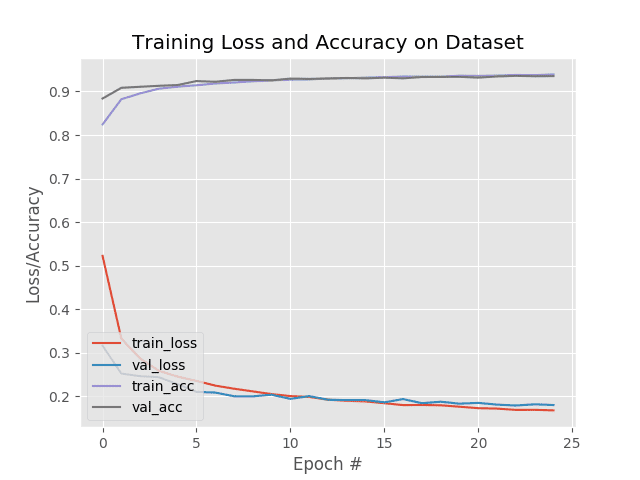
Here you can see that our network obtained 93% accuracy on the testing set.

The model classified the “trouser” class 100% correctly but seemed to struggle quite a bit with the “shirt” class (~81% accurate).

According to our plot in Figure 3, there appears to be very little overfitting.

A deeper architecture with data augmentation would likely lead to higher accuracy.

Below I have included a sample of fashion classifications:

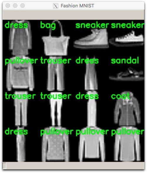
As you can see our network is performing quite well at fashion recognition.

Will this model work for fashion images outside the Fashion MNIST dataset?

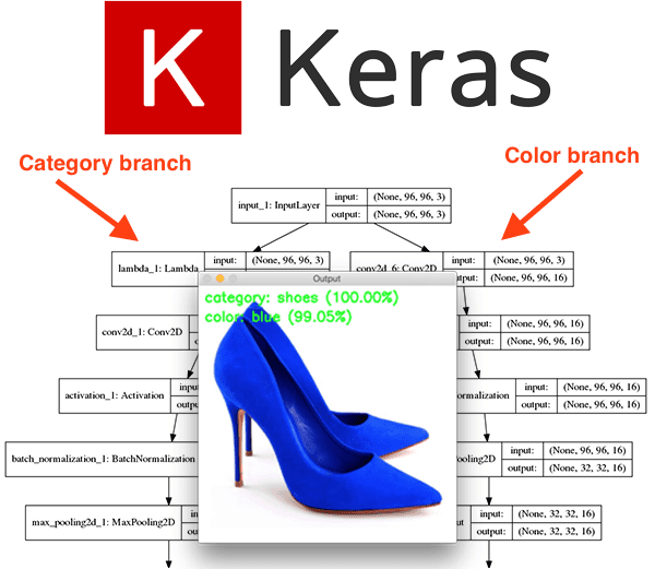
At this point, you are properly wondering if the model we just trained on the Fashion MNIST dataset would be directly applicable to images outside the Fashion MNIST dataset?

The short answer is “No, unfortunately not.”

The longer answer requires a bit of explanation.

To start, keep in mind that the Fashion MNIST dataset is meant to be a drop-in replacement for the MNIST dataset, implying that our images have already been processed.

Each image has been:

• Converted to grayscale.
• Segmented, such that all background pixels are black and all foreground pixels are some gray, non-black pixel intensity.
• Resized to 28×28 pixels.

For real-world fashion and clothing images, you would have to preprocess your data in the same manner as the Fashion MNIST dataset.

And furthermore, even if you could preprocess your dataset in the exact same manner, the model still might not be transferable to real-world images.

Instead, you should train a CNN on example images that will mimic the images the CNN “sees” when deployed to a real-world situation.

To do that you will likely need to utilize multi-label classification and multi-output networks.

For more details on both of these techniques be sure to refer to the following tutorials:

1. Multi-label classification with Keras
2. Keras: Multiple outputs and multiple losses

Summary

In this tutorial, you learned how to train a simple CNN on the Fashion MNIST dataset using Keras.

The Fashion MNIST dataset is meant to be a drop-in replacement for the standard MNIST digit recognition dataset, including:

• 60,000 training examples
• 10,000 testing examples
• 10 classes
• 28×28 grayscale images

While the Fashion MNIST dataset is slightly more challenging than the MNIST digit recognition dataset, unfortunately, it cannot be used directly in real-world fashion classification tasks, unless you preprocess your images in the exact same manner as Fashion MNIST (segmentation, thresholding, grayscale conversion, resizing, etc.).

In most real-world fashion applications mimicking the Fashion MNIST pre-processing steps will be near impossible.

You can and should use Fashion MNIST as a drop-in replacement for the MNIST digit dataset; however, if you are interested in actually recognizing fashion items in real-world images you should refer to the following two tutorials:

1. Multi-label classification with Keras
2. Keras: Multiple outputs and multiple losses

Both of the tutorials linked to above will guide you in building a more robust fashion classification system.

I hope you enjoyed today’s post!

To download the source code to this post, and be notified when future tutorials are published here on PyImageSearch, just enter your email address in the form below!