Keras, Regression, and CNNs

In this tutorial, you will learn how to train a Convolutional Neural Network (CNN) for regression prediction with Keras. You’ll then train a CNN to predict house prices from a set of images.

Today is part two in our three-part series on regression prediction with Keras:

• Part 1: Basic regression with Keras — predicting house prices from categorical and numerical data.
• Part 2: Regression with Keras and CNNs — training a CNN to predict house prices from image data (today’s tutorial).
• Part 3: Combining categorical, numerical, and image data into a single network (next week’s tutorial).

Today’s tutorial builds on last week’s basic Keras regression example, so if you haven’t read it yet make sure you go through it in order to follow along here today.

By the end of this guide, you’ll not only have a strong understanding of training CNNs for regression prediction with Keras, but you’ll also have a Python code template you can follow for your own projects.

To learn how to train a CNN for regression prediction with Keras, just keep reading!

Keras, Regression, and CNNs

2020-06-15 Update: This blog post is now TensorFlow 2+ compatible!

In the first part of this tutorial, we’ll discuss our house prices dataset which consists of not only numerical/categorical data but also image data as well. From there we’ll briefly review our project structure.

We’ll then create two Python helper functions:

1. The first one will be used to load our house price images from disk
2. The second method will be used to construct our Keras CNN architecture

Finally, we’ll implement our training script and then train a Keras CNN for regression prediction.

We’ll also review our results and suggest further methods to improve our prediction accuracy.

Again, I want to reiterate that you should read last week’s tutorial on basic regression prediction before continuing — we’ll be building off not only the concepts from last week but the source code as well.

As you’ll find out in the rest of today’s tutorial, performing regression with CNNs and Keras is as simple as:

1. Removing the fully-connected softmax classifier layer typically used for classification
2. Replacing it with a fully-connected layer with a single node along with a linear activation function.
3. Training the model with a continuous value prediction loss function such as mean squared error, mean absolute error, mean absolute percentage error, etc.

Let’s go ahead get started!

Predicting house prices…with images?

The dataset we’re using for this series of tutorials was curated by Ahmed and Moustafa in their 2016 paper, House price estimation from visual and textual features.

As far as I know, this is the first publicly available dataset that includes both numerical/categorical attributes along with images.

The numerical and categorical attributes include:

1. Number of bedrooms
2. Number of bathrooms
3. Area (i.e., square footage)
4. Zip code

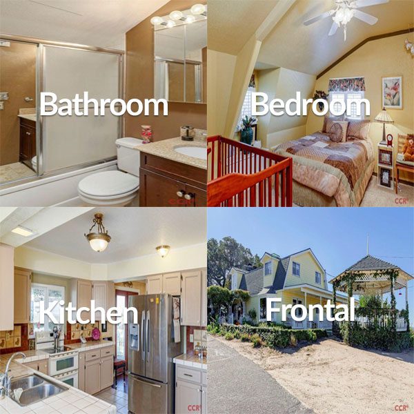
Four images of each house are also provided:

1. Bedroom
2. Bathroom
3. Kitchen
4. Frontal view of the house

A total of 535 houses are included in the dataset, therefore there are 535 x 4 = 2,140 total images in the dataset.

We’ll be pruning that number down to 362 houses (1,448 images) during our data cleaning.

To download the house prices dataset you can just clone Ahmed and Moustafa’s GitHub repository:

$ cd ~
$ git clone https://github.com/emanhamed/Houses-dataset

That single command will download both the numerical/categorical data along with the images themselves.

Make note of where you downloaded the repository on the disk (I put it in my home folder) as you’ll need to supply the path to the repo via command line argument later in this tutorial.

For more information on the house prices dataset please refer to last week’s blog post.

Project structure

Let’s look at the structure of today’s project:

$ tree --dirsfirst
.
├── pyimagesearch
│   ├── __init__.py
│   ├── datasets.py
│   └── models.py
└── cnn_regression.py

1 directory, 4 files

We will be updating both datasets.py and models.py from last week’s tutorial with additional functionality.

Our training script, cnn_regression.py , is completely new this week and it will take advantage of the aforementioned updates.

Loading the house prices image dataset

As we know, our house prices dataset includes four images associated with each house:

1. Bedroom
2. Bathroom
3. Kitchen
4. Frontal view of the house

But how are we going to use these images to train our CNN?

We essentially have three options:

1. Pass the images one at a time through the CNN and use the price of the house as the target value for each image
2. Utilize multiple inputs with Keras and have four independent CNN-like branches that eventually merge into a single output
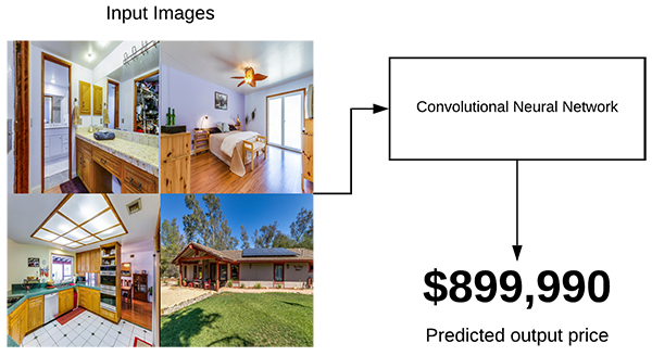
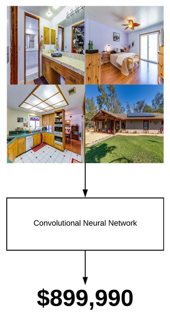
3. Create a montage that combines/tiles all four images into a single image and then pass the montage through the CNN

The first option is a poor choice — we’ll have multiple images with the same target price.

If anything we’re just going to end up “confusing” our CNN, making it impossible for the network to learn how to correlate the prices with the input images.

The second option is also not a good idea — the network will be computationally wasteful and harder to train with four independent tensors as inputs. Each branch will then have its own set of CONV layers that will eventually need to be merged into a single output.

Instead, we should choose the third option where we combine all four images into a single image and then pass that image through the CNN (as depicted in Figure 2 above).

For each house in our dataset, we will create a corresponding tiled image that that includes:

1. The bathroom image in the top-left
2. The bedroom image in the top-right
3. The frontal view in the bottom-right
4. The kitchen in the bottom-left

This tiled image will then be passed through the CNN using the house price as the target predicted value.

The benefit of this approach is that we are:

1. Allowing the CNN to learn from all photos of the house rather than trying to pass the house photos through the CNN one at a time
2. Enabling the CNN to learn discriminative filters from all house photos at once (i.e., not “confusing” the CNN with different images with identical target predicted values)

To learn how we can tile the images for each house, let’s take a look at the load_house_images function in our datasets.py file:

def load_house_images(df, inputPath):
	# initialize our images array (i.e., the house images themselves)
	images = []

	# loop over the indexes of the houses
	for i in df.index.values:
		# find the four images for the house and sort the file paths,
		# ensuring the four are always in the *same order*
		basePath = os.path.sep.join([inputPath, "{}_*".format(i + 1)])
		housePaths = sorted(list(glob.glob(basePath)))

The load_house_images function accepts two parameters:

• df : The houses data frame.
• inputPath : Our dataset path.

Using these parameters, we proceed by initializing a list of images that will be returned to the calling function, once processed.

From there we begin looping (Line 64) over the indexes in our data frame (i.e., one unique index for each house). In the loop we:

• Construct the basePath to the four images for the current index (Line 67).
• Use glob to grab the four image paths (Line 68).

The glob function uses our input path with the wildcard and then finds all input paths that match our pattern.

In the next code block we’re going to populate a list containing the four images:

		# initialize our list of input images along with the output image
		# after *combining* the four input images
		inputImages = []
		outputImage = np.zeros((64, 64, 3), dtype="uint8")

		# loop over the input house paths
		for housePath in housePaths:
			# load the input image, resize it to be 32 32, and then
			# update the list of input images
			image = cv2.imread(housePath)
			image = cv2.resize(image, (32, 32))
			inputImages.append(image)

Continuing in the loop, we proceed to:

• Initialize our inputImages list and allocate memory for our tiled image, outputImage (Lines 72 and 73).
• Create a nested loop over housePaths (Line 76) to load each image , resize to 32×32, and update the inputImages list (Lines 79-81).

And from there, we’ll tile the four images into one montage, eventually returning all of the montages:

		# tile the four input images in the output image such the first
		# image goes in the top-right corner, the second image in the
		# top-left corner, the third image in the bottom-right corner,
		# and the final image in the bottom-left corner
		outputImage[0:32, 0:32] = inputImages[0]
		outputImage[0:32, 32:64] = inputImages[1]
		outputImage[32:64, 32:64] = inputImages[2]
		outputImage[32:64, 0:32] = inputImages[3]

		# add the tiled image to our set of images the network will be
		# trained on
		images.append(outputImage)

	# return our set of images
	return np.array(images)

To finish off the loop, we:

• Tile the input images using NumPy array slicing (Lines 87-90).
• Update images list (Line 94).

Once the process of creating the tiles is done, we go ahead and return the set of images to the calling function on Line 97.

Using Keras to implement a CNN for regression

Let’s go ahead and implement our Keras CNN for regression prediction.

Open up the models.py file and insert the following code:

def create_cnn(width, height, depth, filters=(16, 32, 64), regress=False):
	# initialize the input shape and channel dimension, assuming
	# TensorFlow/channels-last ordering
	inputShape = (height, width, depth)
	chanDim = -1

Our create_cnn function will return our CNN model which we will compile and train in our training script.

The create_cnn function accepts five parameters:

• width : The width of the input images in pixels.
• height : How many pixels tall the input images are.
• depth : The number of channels for the image. For RGB images it is three.
• filters : A tuple of progressively larger filters so that our network can learn more discriminate features.
• regress : A boolean indicating whether or not a fully-connected linear activation layer will be appended to the CNN for regression purposes.

The inputShape of our network is defined on Line 29. It assumes “channels last” ordering for the TensorFlow backend.

Let’s go ahead and define the input to the model and begin creating our CONV => RELU > BN => POOL layer set:

	# define the model input
	inputs = Input(shape=inputShape)

	# loop over the number of filters
	for (i, f) in enumerate(filters):
		# if this is the first CONV layer then set the input
		# appropriately
		if i == 0:
			x = inputs

		# CONV => RELU => BN => POOL
		x = Conv2D(f, (3, 3), padding="same")(x)
		x = Activation("relu")(x)
		x = BatchNormalization(axis=chanDim)(x)
		x = MaxPooling2D(pool_size=(2, 2))(x)

Our model inputs are defined on Line 33.

From there, on Line 36, we loop over the filters and create a set of CONV => RELU > BN => POOL layers. Each iteration of the loop appends these layers. Be sure to check out Chapter 11 from the Starter Bundle of Deep Learning for Computer Vision with Python for more information on these layer types.

Let’s finish building our CNN:

	# flatten the volume, then FC => RELU => BN => DROPOUT
	x = Flatten()(x)
	x = Dense(16)(x)
	x = Activation("relu")(x)
	x = BatchNormalization(axis=chanDim)(x)
	x = Dropout(0.5)(x)

	# apply another FC layer, this one to match the number of nodes
	# coming out of the MLP
	x = Dense(4)(x)
	x = Activation("relu")(x)

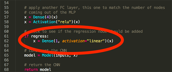
	# check to see if the regression node should be added
	if regress:
		x = Dense(1, activation="linear")(x)

	# construct the CNN
	model = Model(inputs, x)

	# return the CNN
	return model

We Flatten the next layer (Line 49) and then add a fully-connected layer with BatchNormalization and Dropout (Lines 50-53).

Another fully-connected layer is applied to match the four nodes coming out of the multi-layer perceptron (Lines 57 and 58).

On Line 61 and 62, a check is made to see if the regression node should be appended; it is then added it accordingly.

Finally, the model is constructed from our inputs and all the layers we’ve assembled together, x (Line 65).

We can then return the model to the calling function (Line 68).

Implementing the regression training script

Now that we’ve implemented our dataset loader utility function along with our Keras CNN for regression, let’s go ahead and create the training script.

Open up the cnn_regression.py file and insert the following code:

# import the necessary packages
from tensorflow.keras.optimizers import Adam
from sklearn.model_selection import train_test_split
from pyimagesearch import datasets
from pyimagesearch import models
import numpy as np
import argparse
import locale
import os

# construct the argument parser and parse the arguments
ap = argparse.ArgumentParser()
ap.add_argument("-d", "--dataset", type=str, required=True,
	help="path to input dataset of house images")
args = vars(ap.parse_args())

The imports for our training script are taken care of on Lines 2-9. Most notably we’re importing our helper functions from datasets and models . The locale package will help us with formatting our currencies.

From there we parse a single argument using argparse: --dataset . This flag and the argument itself allows us to specify the path to the dataset from our terminal without modifying the script.

Now let’s load, preprocess, and split our data:

# construct the path to the input .txt file that contains information
# on each house in the dataset and then load the dataset
print("[INFO] loading house attributes...")
inputPath = os.path.sep.join([args["dataset"], "HousesInfo.txt"])
df = datasets.load_house_attributes(inputPath)

# load the house images and then scale the pixel intensities to the
# range [0, 1]
print("[INFO] loading house images...")
images = datasets.load_house_images(df, args["dataset"])
images = images / 255.0

# partition the data into training and testing splits using 75% of
# the data for training and the remaining 25% for testing
split = train_test_split(df, images, test_size=0.25, random_state=42)
(trainAttrX, testAttrX, trainImagesX, testImagesX) = split

Our inputPath on Line 20 contains the path to our CSV file containing the numerical and categorical attributes along with the target price for each home.

Our dataset is loaded using the load_house_attributes convenience function we defined in last week’s tutorial (Line 21). The result is a pandas data frame, df , containing the numerical/categorical attributes.

The actual numerical and categorical attributes aren’t used in this tutorial, but we do use the data frame in order to load the images on Line 26 using the convenience function we defined earlier in today’s blog post.

We go ahead and scale our images’ pixel intensities to the range [0, 1] on Line 27.

Then our dataset training and testing splits are constructed using scikit-learn’s handy train_test_split function (Lines 31 and 32).

Again, we will not be using the numerical/categorical data here today, just the images themselves. The numerical/categorical data is used in part one (last week) and part three (next week) of this series.

Now let’s scale our pricing data and train our model:

# find the largest house price in the training set and use it to
# scale our house prices to the range [0, 1] (will lead to better
# training and convergence)
maxPrice = trainAttrX["price"].max()
trainY = trainAttrX["price"] / maxPrice
testY = testAttrX["price"] / maxPrice

# create our Convolutional Neural Network and then compile the model
# using mean absolute percentage error as our loss, implying that we
# seek to minimize the absolute percentage difference between our
# price *predictions* and the *actual prices*
model = models.create_cnn(64, 64, 3, regress=True)
opt = Adam(lr=1e-3, decay=1e-3 / 200)
model.compile(loss="mean_absolute_percentage_error", optimizer=opt)

# train the model
print("[INFO] training model...")
model.fit(x=trainImagesX, y=trainY, 
    validation_data=(testImagesX, testY),
    epochs=200, batch_size=8)

Here we have:

• Scaled the house prices to the range [0, 1] based on the maxPrice (Lines 37-39). Performing this scaling will lead to better training and faster convergence.
• Created and compiled our model using the Adam optimizer (Lines 45-47). We are using mean absolute percentage error as our loss function and we’ve set regress=True indicating that we want to perform regression.
• Kicked of the training process (Lines 51-53).

Now let’s evaluate the results!

# make predictions on the testing data
print("[INFO] predicting house prices...")
preds = model.predict(testImagesX)

# compute the difference between the *predicted* house prices and the
# *actual* house prices, then compute the percentage difference and
# the absolute percentage difference
diff = preds.flatten() - testY
percentDiff = (diff / testY) * 100
absPercentDiff = np.abs(percentDiff)

# compute the mean and standard deviation of the absolute percentage
# difference
mean = np.mean(absPercentDiff)
std = np.std(absPercentDiff)

# finally, show some statistics on our model
locale.setlocale(locale.LC_ALL, "en_US.UTF-8")
print("[INFO] avg. house price: {}, std house price: {}".format(
	locale.currency(df["price"].mean(), grouping=True),
	locale.currency(df["price"].std(), grouping=True)))
print("[INFO] mean: {:.2f}%, std: {:.2f}%".format(mean, std))

In order to evaluate our house prices model based on image data using regression, we:

• Make predictions on test data (Line 57).
• Compute absolute percentage difference (Lines 62-64) and use that to derive our final metrics (Lines 68 and 69).
• Display evaluation information in our terminal (Lines 73-76).

That’s a wrap, but…

Don’t be fooled by how succinct this training script is!

There is a lot going on under the hood with our convenience functions to load the data + create the CNN and the training process which tunes all the weights to the neurons. To brush up on convolutional neural networks, please refer to the Starter Bundle of Deep Learning for Computer Vision with Python.

Training our regression CNN

Ready to train your Keras CNN for regression prediction?

Make sure you have:

1. Configured your development environment according to last week’s tutorial.
2. Used the “Downloads” section of this tutorial to download the source code.
3. Downloaded the house prices dataset using the instructions in the “Predicting house prices…with images?” section above.

From there, open up a terminal and execute the following command:

$ python cnn_regression.py --dataset ~/Houses-dataset/Houses\ Dataset/
[INFO] loading house attributes...
[INFO] loading house images...
[INFO] training model...
Epoch 1/200
34/34 [==============================] - 0s 9ms/step - loss: 1839.4242 - val_loss: 342.6158
Epoch 2/200
34/34 [==============================] - 0s 4ms/step - loss: 1117.5648 - val_loss: 143.6833
Epoch 3/200
34/34 [==============================] - 0s 3ms/step - loss: 682.3041 - val_loss: 188.1647
Epoch 4/200
34/34 [==============================] - 0s 3ms/step - loss: 642.8157 - val_loss: 228.8398
Epoch 5/200
34/34 [==============================] - 0s 3ms/step - loss: 565.1772 - val_loss: 740.4736
Epoch 6/200
34/34 [==============================] - 0s 3ms/step - loss: 460.3651 - val_loss: 1478.7289
Epoch 7/200
34/34 [==============================] - 0s 3ms/step - loss: 365.0139 - val_loss: 1918.3398
Epoch 8/200
34/34 [==============================] - 0s 3ms/step - loss: 368.6264 - val_loss: 2303.6936
Epoch 9/200
34/34 [==============================] - 0s 4ms/step - loss: 377.3214 - val_loss: 1325.1755
Epoch 10/200
34/34 [==============================] - 0s 3ms/step - loss: 266.5995 - val_loss: 1188.1686
...
Epoch 195/200
34/34 [==============================] - 0s 4ms/step - loss: 35.3417 - val_loss: 107.2347
Epoch 196/200
34/34 [==============================] - 0s 3ms/step - loss: 37.4725 - val_loss: 74.4848
Epoch 197/200
34/34 [==============================] - 0s 3ms/step - loss: 38.4116 - val_loss: 102.9308
Epoch 198/200
34/34 [==============================] - 0s 3ms/step - loss: 39.8636 - val_loss: 61.7900
Epoch 199/200
34/34 [==============================] - 0s 3ms/step - loss: 41.9374 - val_loss: 71.8057
Epoch 200/200
34/34 [==============================] - 0s 4ms/step - loss: 40.5261 - val_loss: 67.6559
[INFO] predicting house prices...
[INFO] avg. house price: $533,388.27, std house price: $493,403.08
[INFO] mean: 67.66%, std: 78.06%

Our mean absolute percentage error starts off extremely high, in the order of 300-2,000% in the first ten epochs; however, by the time training is complete we are at a much lower training loss of 40%.

The problem though is that we’ve clearly overfit.

While our training loss is 40% our validation loss is at 67.66%, implying that, on average, our network will be ~68% off in its house price predictions.

How can we improve our prediction accuracy?

Overall, our CNN obtained a mean absolute error of 67.66%, implying, that on average, our CNN will be nearly 68% off in its predicted house value.

That’s a pretty poor result given that our simple MLP trained on the numerical and categorial data obtained a mean absolute error of 22.71%, far better than today’s 67.66%.

So, what does this mean?

Does it mean that CNNs are ill-suited for regression tasks and that we shouldn’t use them for regression?

Actually, no — it doesn’t mean that at all.

Instead, all it means is that the interior of a home doesn’t necessarily correlate with the price of a home.

For example, let’s suppose there is an ultra luxurious celebrity home in Beverly Hills, CA that is valued at $10,000,000.

Now, let’s take that same home and transplant it to Forest Park, one of the worst areas of Detroit.

In this neighborhood the median home price is $13,000 — do you think that gorgeous celebrity house with the decked out interior is still going to be worth $10,000,000?

Of course not.

There is more to the price of a home than just the interior. We also have to factor in the local real estate market itself.

There are a huge number of factors that go into the price of a home but by in large, one of the most important attributes is the locale itself.

Therefore, it shouldn’t be much of a surprise that our CNN trained on house images didn’t perform as well as the simple MLP trained on the numerical and categorical attributes.

But that does raise the question:

1. Is it possible to combine our numerical/categorical data with our image data and train a single end-to-end network?
2. And if so, would our house price prediction accuracy improve?

I’ll answer that question next week, stay tuned.

Summary

In today’s tutorial, you learned how to train a Convolutional Neural Network (CNN) for regression prediction with Keras.

Implementing a CNN for regression prediction is as simple as:

1. Removing the fully-connected softmax classifier layer typically used for classification
2. Replacing it a fully-connected layer with a single node along with a linear activation function.
3. Training the model with continuous value prediction loss function such as mean squared error, mean absolute error, mean absolute percentage error, etc.

What makes this method so powerful is that it implies that we can fine-tune existing models for regression prediction — simply remove the old FC + softmax layer, add in a single node FC layer with a linear activation, update your loss method, and start training!

If you’re interested in learning more about transfer learning and fine-tuning on pre-trained models, please refer to my book, Deep Learning for Computer Vision with Python, where I discuss transfer learning and fine-tuning in detail.

In next week’s tutorial, I’ll be showing you how to work with mixed data using Keras, including combining categorical, numerical, and image data into a single network.

To download the source code to this post, and be notified when next week’s blog post publishes, be sure to enter your email address in the form below!