In this tutorial, you will learn how to perform regression using Keras and Deep Learning. You will learn how to train a Keras neural network for regression and continuous value prediction, specifically in the context of house price prediction.
Today’s post kicks off a 3-part series on deep learning, regression, and continuous value prediction.
We’ll be studying Keras regression prediction in the context of house price prediction:
- Part 1: Today we’ll be training a Keras neural network to predict house prices based on categorical and numerical attributes such as the number of bedrooms/bathrooms, square footage, zip code, etc.
- Part 2: Next week we’ll train a Keras Convolutional Neural Network to predict house prices based on input images of the houses themselves (i.e., frontal view of the house, bedroom, bathroom, and kitchen).
- Part 3: In two weeks we’ll define and train a neural network that combines our categorical/numerical attributes with our images, leading to better, more accurate house price prediction than the attributes or images alone.
Unlike classification (which predicts labels), regression enables us to predict continuous values.
For example, classification may be able to predict one of the following values: {cheap, affordable, expensive}.
Regression, on the other hand, will be able to predict an exact dollar amount, such as “The estimated price of this house is $489,121”.
In many real-world situations, such as house price prediction or stock market forecasting, applying regression rather than classification is critical to obtaining good predictions.
To learn how to perform regression with Keras, just keep reading!
Regression with Keras
2020-06-12 Update: This blog post is now TensorFlow 2+ compatible!
In the first part of this tutorial, we’ll briefly discuss the difference between classification and regression.
We’ll then explore the house prices dataset we’re using for this series of Keras regression tutorials.
From there, we’ll configure our development environment and review our project structure.
Along the way, we will learn how to use Pandas to load our house price dataset and define a neural network that for Keras regression prediction.
Finally, we’ll train our Keras network and then evaluate the regression results.
Classification vs. Regression
Typically on the PyImageSearch blog, we discuss Keras and deep learning in the context of classification — predicting a label to characterize the contents of an image or an input set of data.
Regression, on the other hand, enables us to predict continuous values. Let’s again consider the task of house price prediction.
As we know, classification is used to predict a class label.
For house price prediction we may define our categorical labels as:
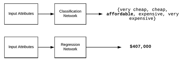
labels = {very cheap, cheap, affordable, expensive, very expensive}
If we performed classification, our model could then learn to predict one of those five values based on a set of input features.
However, those labels are just that — categories that represent a potential range of prices for the house but do nothing to represent the actual cost of the home.
In order to predict the actual cost of a home, we need to perform regression.
Using regression we can train a model to predict a continuous value.
For example, while classification may only be able to predict a label, regression could say:
“Based on my input data, I estimate the cost of this house to be $781,993.”
Figure 1 above provides a visualization of performing both classification and regression.
In the rest of this tutorial, you’ll learn how to train a neural network for regression using Keras.
The House Prices Dataset
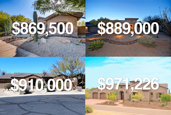
The dataset we’ll be using today is from 2016 paper, House price estimation from visual and textual features, by Ahmed and Moustafa.
The dataset includes both numerical/categorical attributes along with images for 535 data points, making it an excellent dataset to study for regression and mixed data prediction.
The house dataset includes four numerical and categorical attributes:
- Number of bedrooms
- Number of bathrooms
- Area (i.e., square footage)
- Zip code
These attributes are stored on disk in CSV format.
We’ll be loading these attributes from disk later in this tutorial using pandas , a popular Python package used for data analysis.
A total of four images are also provided for each house:
- Bedroom
- Bathroom
- Kitchen
- Frontal view of the house
The end goal of the houses dataset is to predict the price of the home itself.
In today’s tutorial, we’ll be working with just the numerical and categorical data.
Next week’s blog post will discuss working with the image data.
And finally, two weeks from now we’ll combine the numerical/categorical data with the images to obtain our best performing model.
But before we can train our Keras model for regression, we first need to configure our development environment and grab the data.
Configuring Your Development Environment
For this 3-part series of blog posts, you’ll need to have the following packages installed:
- NumPy
- scikit-learn
- pandas
- Keras with the TensorFlow backend (CPU or GPU)
- OpenCV (for the next two blog posts in the series)
To configure your system for this series of tutorials, I recommend following either of these tutorials:
Either tutorial will help you configure you system with all the necessary software for this blog post in a convenient Python virtual environment.
Please note that PyImageSearch does not recommend or support Windows for CV/DL projects.
Downloading the House Prices Dataset
Before you download the dataset, go ahead and grab the source code to this post by using “Downloads” section.
From there, unzip the file and navigate into the directory:
$ cd path/to/downloaded/zip
$ unzip keras-regression.zip
$ cd keras-regression
From there, you can download the House Prices Dataset using the following command:
$ git clone https://github.com/emanhamed/Houses-dataset
When we are ready to train our Keras regression network you’ll then need to supply the path to the Houses-dataset directory via command line argument.
Project structure
Now that you have the dataset, go ahead and use the tree command with the same arguments shown below to print a directory + file listing for the project:
$ tree --dirsfirst --filelimit 10
.
├── Houses-dataset
│   ├── Houses Dataset [2141 entries]
│   └── README.md
├── pyimagesearch
│   ├── __init__.py
│   ├── datasets.py
│   └── models.py
└── mlp_regression.py

3 directories, 5 files
The dataset downloaded from GitHub now resides in the Houses-dataset/ folder.
The pyimagesearch/ directory is actually a module included with the code “Downloads” where inside, you’ll find:
datasets.py: Our script for loading the numerical/categorical data from the datasetmodels.py: Our Multi-Layer Perceptron architecture implementation
These two scripts will be reviewed today. Additionally, we’ll be reusing both datasets.py and models.py (with modifications) in the next two tutorials to keep our code organized and reusable.
The regression + Keras script is contained in mlp_regression.py which we’ll be reviewing it as well.
Loading the House Prices Dataset
Before we can train our Keras regression model we first need to load the numerical and categorical data for the houses dataset.
Open up the datasets.py file and insert the following code:
# import the necessary packages
from sklearn.preprocessing import LabelBinarizer
from sklearn.preprocessing import MinMaxScaler
import pandas as pd
import numpy as np
import glob
import cv2
import os

def load_house_attributes(inputPath):
	# initialize the list of column names in the CSV file and then
	# load it using Pandas
	cols = ["bedrooms", "bathrooms", "area", "zipcode", "price"]
	df = pd.read_csv(inputPath, sep=" ", header=None, names=cols)
We begin by importing libraries and modules from scikit-learn, pandas, NumPy and OpenCV. OpenCV will be used next week as we’ll be adding the ability to load images to this script.
On Line 10, we define the load_house_attributes function which accepts the path to the input dataset.
Inside the function we start off by defining the names of the columns in the CSV file (Line 13). From there, we use pandas’ function, read_csv to load the CSV file into memory as a date frame ( df ) on Line 14.
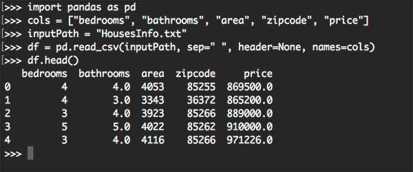
Below you can see an example of our input data, including the number of bedrooms, number of bathrooms, area (i.e., square footage), zip code, code, and finally the target price our model should be trained to predict:
   bedrooms  bathrooms  area  zipcode     price
0         4        4.0  4053    85255  869500.0
1         4        3.0  3343    36372  865200.0
2         3        4.0  3923    85266  889000.0
3         5        5.0  4022    85262  910000.0
4         3        4.0  4116    85266  971226.0
Let’s finish up the rest of the load_house_attributes function:
	# determine (1) the unique zip codes and (2) the number of data
	# points with each zip code
	zipcodes = df["zipcode"].value_counts().keys().tolist()
	counts = df["zipcode"].value_counts().tolist()

	# loop over each of the unique zip codes and their corresponding
	# count
	for (zipcode, count) in zip(zipcodes, counts):
		# the zip code counts for our housing dataset is *extremely*
		# unbalanced (some only having 1 or 2 houses per zip code)
		# so let's sanitize our data by removing any houses with less
		# than 25 houses per zip code
		if count < 25:
			idxs = df[df["zipcode"] == zipcode].index
			df.drop(idxs, inplace=True)

	# return the data frame
	return df
In the remaining lines, we:
- Determine the unique set of zip codes and then count the number of data points with each unique zip code (Lines 18 and 19).
- Filter out zip codes with low counts (Line 28). For some zip codes we only have one or two data points, making it extremely challenging, if not impossible, to obtain accurate house price estimates.
- Return the data frame to the calling function (Line 33).
Now let’s create the process_house_attributes function used to preprocess our data:
def process_house_attributes(df, train, test):
	# initialize the column names of the continuous data
	continuous = ["bedrooms", "bathrooms", "area"]

	# performin min-max scaling each continuous feature column to
	# the range [0, 1]
	cs = MinMaxScaler()
	trainContinuous = cs.fit_transform(train[continuous])
	testContinuous = cs.transform(test[continuous])
We define the function on Line 35. The process_house_attributes function accepts three parameters:
df: Our data frame generated by pandas (the previous function helps us to drop some records from the data frame)train: Our training data for the House Prices Datasettest: Our testing data.
Then on Line 37, we define the columns of our continuous data, including bedrooms, bathrooms, and size of the home.
We’ll take these values and use scikit-learn’s MinMaxScaler to scale the continuous features to the range [0, 1] (Lines 41-43).
Now we need to pre-process our categorical features, namely the zip code:
	# one-hot encode the zip code categorical data (by definition of
	# one-hot encoing, all output features are now in the range [0, 1])
	zipBinarizer = LabelBinarizer().fit(df["zipcode"])
	trainCategorical = zipBinarizer.transform(train["zipcode"])
	testCategorical = zipBinarizer.transform(test["zipcode"])

	# construct our training and testing data points by concatenating
	# the categorical features with the continuous features
	trainX = np.hstack([trainCategorical, trainContinuous])
	testX = np.hstack([testCategorical, testContinuous])

	# return the concatenated training and testing data
	return (trainX, testX)
First, we’ll one-hot encode the zip codes (Lines 47-49).
Then we’ll concatenate the categorical features with the continuous features using NumPy’s hstack function (Lines 53 and 54), returning the resulting training and testing sets as a tuple (Line 57).
Keep in mind that now both our categorical features and continuous features are all in the range [0, 1].
Implementing a Neural Network for Regression
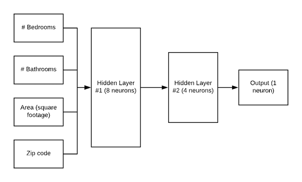
Before we can train a Keras network for regression, we first need to define the architecture itself.
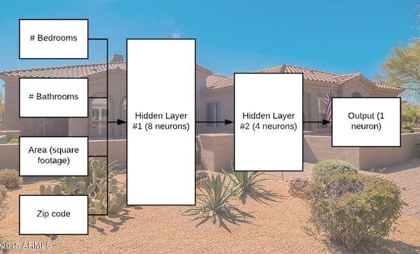
Today we’ll be using a simple Multilayer Perceptron (MLP) as shown in Figure 5.
Open up the models.py file and insert the following code:
# import the necessary packages
from tensorflow.keras.models import Sequential
from tensorflow.keras.layers import BatchNormalization
from tensorflow.keras.layers import Conv2D
from tensorflow.keras.layers import MaxPooling2D
from tensorflow.keras.layers import Activation
from tensorflow.keras.layers import Dropout
from tensorflow.keras.layers import Dense
from tensorflow.keras.layers import Flatten
from tensorflow.keras.layers import Input
from tensorflow.keras.models import Model

def create_mlp(dim, regress=False):
	# define our MLP network
	model = Sequential()
	model.add(Dense(8, input_dim=dim, activation="relu"))
	model.add(Dense(4, activation="relu"))

	# check to see if the regression node should be added
	if regress:
		model.add(Dense(1, activation="linear"))

	# return our model
	return model
First, we’ll import all of the necessary modules from Keras (Lines 2-11). We’ll be adding a Convolutional Neural Network to this file in next week’s tutorial, hence the additional imports that aren’t utilized here today.
Let’s define the MLP architecture by writing a function to generate it called create_mlp .
The function accepts two parameters:
dim: Defines our input dimensionsregress: A boolean defining whether or not our regression neuron should be added
We’ll go ahead and start construction our MLP with a dim-8-4 architecture (Lines 15-17).
If we are performing regression, we add a Dense layer containing a single neuron with a linear activation function (Lines 20 and 21). Typically we use ReLU-based activations, but since we are performing regression we need a linear activation.
Finally, our model is returned on Line 24.
Implementing our Keras Regression Script
It’s now time to put all the pieces together!
Open up the mlp_regression.py file and insert the following code:
# import the necessary packages
from tensorflow.keras.optimizers import Adam
from sklearn.model_selection import train_test_split
from pyimagesearch import datasets
from pyimagesearch import models
import numpy as np
import argparse
import locale
import os

# construct the argument parser and parse the arguments
ap = argparse.ArgumentParser()
ap.add_argument("-d", "--dataset", type=str, required=True,
	help="path to input dataset of house images")
args = vars(ap.parse_args())
We begin by importing necessary packages, modules, and libraries.
Namely, we’ll need the Adam optimizer from Keras, train_test_split from scikit-learn, and our datasets + models functions from the pyimagesearch module.
Additionally, we’ll use math features from NumPy for collecting statistics when we evaluate our model.
The argparse module is for parsing command line arguments.
Our script requires just one command line argument --dataset (Lines 12-15). You’ll need to provide the --dataset switch and the actual path to the dataset when you go to run the training script in your terminal.
Let’s load the house dataset attributes and construct our training and testing splits:
# construct the path to the input .txt file that contains information
# on each house in the dataset and then load the dataset
print("[INFO] loading house attributes...")
inputPath = os.path.sep.join([args["dataset"], "HousesInfo.txt"])
df = datasets.load_house_attributes(inputPath)

# construct a training and testing split with 75% of the data used
# for training and the remaining 25% for evaluation
print("[INFO] constructing training/testing split...")
(train, test) = train_test_split(df, test_size=0.25, random_state=42)
Using our handy load_house_attributes function, and by passing the inputPath to the dataset itself, our data is loaded into memory (Lines 20 and 21).
Our training (75%) and testing (25%) data is constructed via Line 26 and scikit-learn’s train_test_split method.
Let’s scale our house pricing data:
# find the largest house price in the training set and use it to
# scale our house prices to the range [0, 1] (this will lead to
# better training and convergence)
maxPrice = train["price"].max()
trainY = train["price"] / maxPrice
testY = test["price"] / maxPrice
As stated in the comment, scaling our house prices to the range [0, 1] will allow our model to more easily train and converge. Scaling the output targets to [0, 1] will reduce the range of our output predictions (versus [0, maxPrice ]) and make it not only easier and faster to train our network but enable our model to obtain better results as well.
Thus, we grab the maximum price in the training set (Line 31), and proceed to scale our training and testing data accordingly (Lines 32 and 33).
Let’s process the house attributes now:
# process the house attributes data by performing min-max scaling
# on continuous features, one-hot encoding on categorical features,
# and then finally concatenating them together
print("[INFO] processing data...")
(trainX, testX) = datasets.process_house_attributes(df, train, test)
Recall from the datasets.py script that the process_house_attributes function:
- Pre-processes our categorical and continuous features.
- Scales our continuous features to the range [0, 1] via min-max scaling.
- One-hot encodes our categorical features.
- Concatenates the categorical and continuous features to form the final feature vector.
Now let’s go ahead and fit our MLP model to the data:
# create our MLP and then compile the model using mean absolute
# percentage error as our loss, implying that we seek to minimize
# the absolute percentage difference between our price *predictions*
# and the *actual prices*
model = models.create_mlp(trainX.shape[1], regress=True)
opt = Adam(lr=1e-3, decay=1e-3 / 200)
model.compile(loss="mean_absolute_percentage_error", optimizer=opt)

# train the model
print("[INFO] training model...")
model.fit(x=trainX, y=trainY,
	validation_data=(testX, testY),
	epochs=200, batch_size=8)
Our model is initialized with the Adam optimizer (Lines 45 and 46) and then compiled (Line 47). Notice that we’re using mean absolute percentage error as our loss function, indicating that we seek to minimize the mean percentage difference between the predicted price and the actual price.
The actual training process is kicked off on Lines 51-53.
After training is complete we can evaluate our model and summarize our results:
# make predictions on the testing data
print("[INFO] predicting house prices...")
preds = model.predict(testX)

# compute the difference between the *predicted* house prices and the
# *actual* house prices, then compute the percentage difference and
# the absolute percentage difference
diff = preds.flatten() - testY
percentDiff = (diff / testY) * 100
absPercentDiff = np.abs(percentDiff)

# compute the mean and standard deviation of the absolute percentage
# difference
mean = np.mean(absPercentDiff)
std = np.std(absPercentDiff)

# finally, show some statistics on our model
locale.setlocale(locale.LC_ALL, "en_US.UTF-8")
print("[INFO] avg. house price: {}, std house price: {}".format(
	locale.currency(df["price"].mean(), grouping=True),
	locale.currency(df["price"].std(), grouping=True)))
print("[INFO] mean: {:.2f}%, std: {:.2f}%".format(mean, std))
Line 57 instructs Keras to make predictions on our testing set.
Using the predictions, we compute the:
- Difference between predicted house prices and the actual house prices (Line 62).
- Percentage difference (Line 63).
- Absolute percentage difference (Line 64).
From there, on Lines 68 and 69, we calculate the mean and standard deviation of the absolute percentage difference.
The results are printed via Lines 73-76.
Regression with Keras wasn’t so tough, now was it?
Let’s train the model and analyze the results!
Keras Regression Results

To train our own Keras network for regression and house price prediction make sure you have:
- Configured your development environment according to the guidance above.
- Used the “Downloads” section of this tutorial to download the source code.
- Downloaded the house prices dataset based on the instructions in the “The House Prices Dataset” section above.
From there, open up a terminal and supply the following command (making sure the --dataset command line argument points to where you downloaded the house prices dataset):
$ python mlp_regression.py --dataset Houses-dataset/Houses\ Dataset/
[INFO] loading house attributes...
[INFO] constructing training/testing split...
[INFO] processing data...
[INFO] training model...
Epoch 1/200
34/34 [==============================] - 0s 4ms/step - loss: 73.0898 - val_loss: 63.0478
Epoch 2/200
34/34 [==============================] - 0s 2ms/step - loss: 58.0629 - val_loss: 56.4558
Epoch 3/200
34/34 [==============================] - 0s 1ms/step - loss: 51.0134 - val_loss: 50.1950
Epoch 4/200
34/34 [==============================] - 0s 1ms/step - loss: 47.3431 - val_loss: 47.6673
Epoch 5/200
34/34 [==============================] - 0s 1ms/step - loss: 45.5581 - val_loss: 44.9802
Epoch 6/200
34/34 [==============================] - 0s 1ms/step - loss: 42.4403 - val_loss: 41.0660
Epoch 7/200
34/34 [==============================] - 0s 1ms/step - loss: 39.5451 - val_loss: 34.4310
Epoch 8/200
34/34 [==============================] - 0s 2ms/step - loss: 34.5027 - val_loss: 27.2138
Epoch 9/200
34/34 [==============================] - 0s 2ms/step - loss: 28.4326 - val_loss: 25.1955
Epoch 10/200
34/34 [==============================] - 0s 2ms/step - loss: 28.3634 - val_loss: 25.7194
...
Epoch 195/200
34/34 [==============================] - 0s 2ms/step - loss: 20.3496 - val_loss: 22.2558
Epoch 196/200
34/34 [==============================] - 0s 2ms/step - loss: 20.4404 - val_loss: 22.3071
Epoch 197/200
34/34 [==============================] - 0s 2ms/step - loss: 20.0506 - val_loss: 21.8648
Epoch 198/200
34/34 [==============================] - 0s 2ms/step - loss: 20.6169 - val_loss: 21.5130
Epoch 199/200
34/34 [==============================] - 0s 2ms/step - loss: 19.9067 - val_loss: 21.5018
Epoch 200/200
34/34 [==============================] - 0s 2ms/step - loss: 19.9570 - val_loss: 22.7063
[INFO] predicting house prices...
[INFO] avg. house price: $533,388.27, std house price: $493,403.08
[INFO] mean: 22.71%, std: 18.26%
As you can see from our output, our initial mean absolute percentage error starts off as high as 73% and then quickly drops to under 30%.
By the time we finish training we can see our network starting to overfit a bit. Our training loss is as low as ~20%; however, our validation loss is at ~23%.
Computing our final mean absolute percentage error we obtain a final value of 22.71%.
What does this value mean?
Our final mean absolute percentage error implies, that on average, our network will be ~23% off in its house price predictions with a standard deviation of ~18%.
Limitations of the House Price Dataset
Being 22% off in a house price prediction is a good start but is certainly not the type of accuracy we are looking for.
That said, this prediction accuracy can also be seen as a limitation of the house price dataset itself.
Keep in mind that the dataset only includes four attributes:
- Number of bedrooms
- Number of bathrooms
- Area (i.e., square footage)
- Zip code
Most other house price datasets include many more attributes.
For example, the Boston House Prices Dataset includes a total of fourteen attributes which can be leveraged for house price prediction (although that dataset does have some racial discrimination).
The Ames House Dataset includes over 79 different attributes which can be used to train regression models.
When you think about it, the fact that we are able to even obtain 26% mean absolute percentage error without the knowledge of an expert real estate agent is fairly reasonable given:
- There are only 535 total houses in the dataset (we only used 362 total houses for the purpose of this guide).
- We only have four attributes to train our regression model on.
- The attributes themselves, while important in describing the home itself, do little to characterize the area surrounding the house.
- The house prices are incredibly varied with a mean of $533K and a standard deviation of $493K (based on our filtered dataset of 362 homes).
With all that said, learning how to perform regression with Keras is an important skill!
In the next two posts in this series I’ll be showing you how to:
- Leverage the images provided with the house price dataset to train a CNN on them.
- Combine our numerical/categorical data with the house images, leading to a model that outperforms all of our previous Keras regression experiments.
What's next? We recommend PyImageSearch University.
86+ total classes • 115+ hours hours of on-demand code walkthrough videos • Last updated: May 2026
★★★★★ 4.84 (128 Ratings) • 16,000+ Students Enrolled
I strongly believe that if you had the right teacher you could master computer vision and deep learning.
Do you think learning computer vision and deep learning has to be time-consuming, overwhelming, and complicated? Or has to involve complex mathematics and equations? Or requires a degree in computer science?
That’s not the case.
All you need to master computer vision and deep learning is for someone to explain things to you in simple, intuitive terms. And that’s exactly what I do. My mission is to change education and how complex Artificial Intelligence topics are taught.
If you're serious about learning computer vision, your next stop should be PyImageSearch University, the most comprehensive computer vision, deep learning, and OpenCV course online today. Here you’ll learn how to successfully and confidently apply computer vision to your work, research, and projects. Join me in computer vision mastery.
Inside PyImageSearch University you'll find:
- ✓ 86+ courses on essential computer vision, deep learning, and OpenCV topics
- ✓ 86 Certificates of Completion
- ✓ 115+ hours hours of on-demand video
- ✓ Brand new courses released regularly, ensuring you can keep up with state-of-the-art techniques
- ✓ Pre-configured Jupyter Notebooks in Google Colab
- ✓ Run all code examples in your web browser — works on Windows, macOS, and Linux (no dev environment configuration required!)
- ✓ Access to centralized code repos for all 540+ tutorials on PyImageSearch
- ✓ Easy one-click downloads for code, datasets, pre-trained models, etc.
- ✓ Access on mobile, laptop, desktop, etc.
Summary
In this tutorial, you learned how to use the Keras deep learning library for regression.
Specifically, we used Keras and regression to predict the price of houses based on four numerical and categorical attributes:
- Number of bedrooms
- Number of bathrooms
- Area (i.e., square footage)
- Zip code
Overall our neural network obtained a mean absolute percentage error of 22.71%, implying that, on average, our house price predictions will be off by 22.71%.
That raises the questions:
- How can we better our house price prediction accuracy?
- What if we leveraged images for each house? Would that improve accuracy?
- Is there some way to combine both our categorical/numerical attributes with our image data?
To answer these questions you’ll need to stay tuned for the remaining to tutorials in this Keras regression series.
To download the source code to this post (and be notified when the next tutorial is published here on PyImageSearch), just enter your email address in the form below.

Download the Source Code and FREE 17-page Resource Guide
Enter your email address below to get a .zip of the code and a FREE 17-page Resource Guide on Computer Vision, OpenCV, and Deep Learning. Inside you'll find my hand-picked tutorials, books, courses, and libraries to help you master CV and DL!
