Machine Learning in Python

Struggling to get started with machine learning using Python? In this step-by-step, hands-on tutorial you will learn how to perform machine learning using Python on numerical data and image data.

By the time you are finished reading this post, you will be able to get your start in machine learning.

To effectively understand machine learning in Python, a dataset containing patterns that can be learned by a machine learning algorithm is vital. The right dataset will demonstrate the power of machine learning in discerning patterns and making predictions.

Roboflow has free tools for each stage of the computer vision pipeline that will streamline your workflows and supercharge your productivity.

Sign up or Log in to your Roboflow account to access state of the art dataset libaries and revolutionize your computer vision pipeline.

You can start by choosing your own datasets or using our PyimageSearch’s assorted library of useful datasets.

Bring data in any of 40+ formats to Roboflow, train using any state-of-the-art model architectures, deploy across multiple platforms (API, NVIDIA, browser, iOS, etc), and connect to applications or 3rd party tools.

To launch your machine learning in Python education, just keep reading!

Machine Learning in Python

Inside this tutorial, you will learn how to perform machine learning in Python on numerical data and image data.

You will learn how to operate popular Python machine learning and deep learning libraries, including two of my favorites:

• scikit-learn
• Keras

Specifically, you will learn how to:

1. Examine your problem
2. Prepare your data (raw data, feature extraction, feature engineering, etc.)
3. Spot-check a set of algorithms
4. Examine your results
5. Double-down on the algorithms that worked best

Using this technique you will be able to get your start with machine learning and Python!

Along the way, you’ll discover popular machine learning algorithms that you can use in your own projects as well, including:

1. k-Nearest Neighbors (k-NN)
2. Naïve Bayes
3. Logistic Regression
4. Support Vector Machines (SVMs)
5. Decision Trees
6. Random Forests
7. Perceptrons
8. Multi-layer, feedforward neural networks
9. Convolutional Neural Networks (CNNs)

This hands-on experience will give you the knowledge (and confidence) you need to apply machine learning in Python to your own projects.

Install the required Python machine learning libraries

Before we can get started with this tutorial you first need to make sure your system is configured for machine learning. Today’s code requires the following libraries:

• NumPy: For numerical processing with Python.
• PIL: A simple image processing library.
• scikit-learn: Contains the machine learning algorithms we’ll cover today (we’ll need version 0.20+ which is why you see the --upgrade flag below).
• Keras and TensorFlow: For deep learning. The CPU version of TensorFlow is fine for today’s example.
• OpenCV: While we aren’t using OpenCV for this blog post, imutils depends upon it (next bullet). Because of this, you can simply use pip to install OpenCV, just bear in mind that you won’t have the full install of OpenCV and you can’t customize it.
• imutils: My personal package of image processing/computer vision convenience functions

Each of these can be installed in your environment (virtual environments recommended) with pip:

$ pip install numpy
$ pip install pillow
$ pip install --upgrade scikit-learn
$ pip install tensorflow # or tensorflow-gpu
$ pip install keras
$ pip install opencv-contrib-python
$ pip install --upgrade imutils

Datasets

In order to help you gain experience performing machine learning in Python, we’ll be working with two separate datasets.

The first one, the Iris dataset, is the machine learning practitioner’s equivalent of “Hello, World!” (likely one of the first pieces of software you wrote when learning how to program).

The second dataset, 3-scenes, is an example image dataset I put together — this dataset will help you gain experience working with image data, and most importantly, learn what techniques work best for numerical/categorical datasets vs. image datasets.

Let’s go ahead and get a more intimate look at these datasets.

The Iris dataset

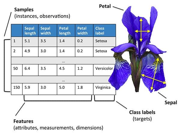
The Iris dataset is arguably one of the most simplistic machine learning datasets — it is often used to help teach programmers and engineers the fundamentals of machine learning and pattern recognition.

We call this dataset the “Iris dataset” because it captures attributes of three Iris flower species:

1. Iris Setosa
2. Iris Versicolor
3. Iris Virginica

Each species of flower is quantified via four numerical attributes, all measured in centimeters:

1. Sepal length
2. Sepal width
3. Petal length
4. Petal width

Our goal is to train a machine learning model to correctly predict the flower species from the measured attributes.

It’s important to note that one of the classes is linearly separable from the other two — the latter are not linearly separable from each other.

In order to correctly classify these the flower species, we will need a non-linear model.

It’s extremely common to need a non-linear model when performing machine learning with Python in the real world — the rest of this tutorial will help you gain this experience and be more prepared to conduct machine learning on your own datasets.

The 3-scenes image dataset

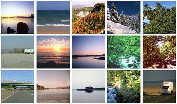
The second dataset we’ll be using to train machine learning models is called the 3-scenes dataset and includes 948 total images of 3 scenes:

• Coast (360 of images)
• Forest (328 of images)
• Highway (260 of images)

The 3-scenes dataset was created by sampling the 8-scenes dataset from Oliva and Torralba’s 2001 paper, Modeling the shape of the scene: a holistic representation of the spatial envelope.

Our goal will be to train machine learning and deep learning models with Python to correctly recognize each of these scenes.

I have included the 3-scenes dataset in the “Downloads” section of this tutorial. Make sure you download the dataset + code to this blog post before continuing.

Steps to perform machine learning in Python

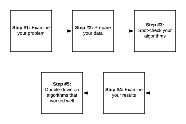
Whenever you perform machine learning in Python I recommend starting with a simple 5-step process:

1. Examine your problem
2. Prepare your data (raw data, feature extraction, feature engineering, etc.)
3. Spot-check a set of algorithms
4. Examine your results
5. Double-down on the algorithms that worked best

This pipeline will evolve as your machine learning experience grows, but for beginners, this is the machine learning process I recommend for getting started.

To start, we must examine the problem.

Ask yourself:

• What type of data am I working with? Numerical? Categorical? Images?
• What is the end goal of my model?
• How will I define and measure “accuracy”?
• Given my current knowledge of machine learning, do I know any algorithms that work well on these types of problems?

The last question, in particular, is critical — the more you apply machine learning in Python, the more experience you will gain.

Based on your previous experience you may already know an algorithm that works well.

From there, you need to prepare your data.

Typically this step involves loading your data from disk, examining it, and deciding if you need to perform feature extraction or feature engineering.

Feature extraction is the process of applying an algorithm to quantify your data in some manner.

For example, when working with images we may wish to compute histograms to summarize the distribution of pixel intensities in the image — in this manner, we can characterize the color of the image.

Feature engineering, on the other hand, is the process of transforming your raw input data into a representation that better represents the underlying problem.

Feature engineering is a more advanced technique and one I recommend you explore once you already have some experience with machine learning and Python.

Next, you’ll want to spot-check a set of algorithms.

What do I mean by spot-checking?

Simply take a set of machine learning algorithms and apply them to the dataset!

You’ll likely want to stuff the following machine learning algorithms in your toolbox:

1. A linear model (ex. Logistic Regression, Linear SVM),
2. A few non-linear models (ex. RBF SVMs, SGD classifiers),
3. Some tree and ensemble-based models (ex. Decision Trees, Random Forests).
4. A few neural networks, if applicable (Multi-layer Perceptrons, Convolutional Neural Networks)

Try to bring a robust set of machine learning models to the problem — your goal here is to gain experience on your problem/project by identifying which machine learning algorithms performed well on the problem and which ones did not.

Once you’ve defined your set of models, train them and evaluate the results.

Which machine learning models worked well? Which models performed poorly?

Take your results and use them to double-down your efforts on the machine learning models that performed while discarding the ones that didn’t.

Over time you will start to see patterns emerge across multiple experiments and projects.

You’ll start to develop a “sixth sense” of what machine learning algorithms perform well and in what situation.

For example, you may discover that Random Forests work very well when applied to projects that have many real-valued features.

On the other hand, you might note that Logistic Regression can handle sparse, high-dimensional spaces well.

You may even find that Convolutional Neural Networks work great for image classification (which they do).

Use your knowledge here to supplement traditional machine learning education — the best way to learn machine learning with Python is to simply roll up your sleeves and get your hands dirty!

A machine learning education based on practical experience (supplemented with some super basic theory) will take you a long way on your machine learning journey!

Let’s get our hands dirty!

Now that we have discussed the fundamentals of machine learning, including the steps required to perform machine learning in Python, let’s get our hands dirty.

In the next section, we’ll briefly review our directory and project structure for this tutorial.

Note: I recommend you use the “Downloads” section of the tutorial to download the source code and example data so you can easily follow along.

Once we’ve reviewed the directory structure for the machine learning project we will implement two Python scripts:

1. The first script will be used to train machine learning algorithms on numerical data (i.e., the Iris dataset)
2. The second Python script will be utilized to train machine learning on image data (i.e., the 3-scenes dataset)

As a bonus we’ll implement two more Python scripts, each of these dedicated to neural networks and deep learning:

1. We’ll start by implementing a Python script that will train a neural network on the Iris dataset
2. Secondly, you’ll learn how to train your first Convolutional Neural Network on the 3-scenes dataset

Let’s get started by first reviewing our project structure.

Our machine learning project structure

Be sure to grab the “Downloads” associated with this blog post.

From there you can unzip the archive and inspect the contents:

$ tree --dirsfirst --filelimit 10
.
├── 3scenes
│   ├── coast [360 entries]
│   ├── forest [328 entries]
│   └── highway [260 entries]
├── classify_iris.py
├── classify_images.py
├── nn_iris.py
└── basic_cnn.py

4 directories, 4 files

The Iris dataset is built into scikit-learn. The 3-scenes dataset, however, is not. I’ve included it in the 3scenes/ directory and as you can see there are three subdirectories (classes) of images.

We’ll be reviewing four Python machine learning scripts today:

• classify_iris.py : Loads the Iris dataset and can apply any one of seven machine learning algorithms with a simple command line argument switch.
• classify_images.py : Gathers our image dataset (3-scenes) and applies any one of seven Python machine learning algorithms
• nn_iris.py : Applies a simple multi-layer neural network to the Iris dataset
• basic_cnn.py : Builds a Convolutional Neural Network (CNN) and trains a model using the 3-scenes dataset

Implementing Python machine learning for numerical data

The first script we are going to implement is classify_iris.py — this script will be used to spot-check machine learning algorithms on the Iris dataset.

Once implemented, we’ll be able to use classify_iris.py to run a suite of machine learning algorithms on the Iris dataset, look at the results, and decide on which algorithm works best for the project.

Let’s get started — open up the classify_iris.py file and insert the following code:

# import the necessary packages
from sklearn.neighbors import KNeighborsClassifier
from sklearn.naive_bayes import GaussianNB
from sklearn.linear_model import LogisticRegression
from sklearn.svm import SVC
from sklearn.tree import DecisionTreeClassifier
from sklearn.ensemble import RandomForestClassifier
from sklearn.neural_network import MLPClassifier
from sklearn.model_selection import train_test_split
from sklearn.metrics import classification_report
from sklearn.datasets import load_iris
import argparse

# construct the argument parser and parse the arguments
ap = argparse.ArgumentParser()
ap.add_argument("-m", "--model", type=str, default="knn",
	help="type of python machine learning model to use")
args = vars(ap.parse_args())

Lines 2-12 import our required packages, specifically:

• Our Python machine learning methods from scikit-learn (Lines 2-8)
• A dataset splitting method used to separate our data into training and testing subsets (Line 9)
• The classification report utility from scikit-learn which will print a summarization of our machine learning results (Line 10)
• Our Iris dataset, built into scikit-learn (Line 11)
• A tool for command line argument parsing called argparse (Line 12)

Using argparse , let’s parse a single command line argument flag, --model on Lines 15-18. The --model switch allows us to choose from any of the following models:

# define the dictionary of models our script can use, where the key
# to the dictionary is the name of the model (supplied via command
# line argument) and the value is the model itself
models = {
	"knn": KNeighborsClassifier(n_neighbors=1),
	"naive_bayes": GaussianNB(),
	"logit": LogisticRegression(solver="lbfgs", multi_class="auto"),
	"svm": SVC(kernel="rbf", gamma="auto"),
	"decision_tree": DecisionTreeClassifier(),
	"random_forest": RandomForestClassifier(n_estimators=100),
	"mlp": MLPClassifier()
}

The models dictionary on Lines 23-31 defines the suite of models we will be spot-checking (we’ll review the results of each of these algorithms later in the post):

• k-Nearest Neighbor (k-NN)
• Naïve Bayes
• Logistic Regression
• Support Vector Machines (SVMs)
• Decision Trees
• Random Forests
• Perceptrons

The keys can be entered directly in the terminal following the --model switch. Here’s an example:

$ python classify_irs.py --model knn

From there the KNeighborClassifier will be loaded automatically. This conveniently allows us to call any one of 7 machine learning models one-at-a-time and on demand in a single Python script (no editing the code required)!

Moving on, let’s load and split our data:

# load the Iris dataset and perform a training and testing split,
# using 75% of the data for training and 25% for evaluation
print("[INFO] loading data...")
dataset = load_iris()
(trainX, testX, trainY, testY) = train_test_split(dataset.data,
	dataset.target, random_state=3, test_size=0.25)

Our dataset is easily loaded with the dedicated load_iris method on Line 36. Once the data is in memory, we go ahead and call train_test_split to separate the data into 75% for training and 25% for testing (Lines 37 and 38).

The final step is to train and evaluate our model:

# train the model
print("[INFO] using '{}' model".format(args["model"]))
model = models[args["model"]]
model.fit(trainX, trainY)

# make predictions on our data and show a classification report
print("[INFO] evaluating...")
predictions = model.predict(testX)
print(classification_report(testY, predictions,
	target_names=dataset.target_names))

Lines 42 and 43 train the Python machine learning model (also known as “fitting a model”, hence the call to .fit ).

From there, we evaluate the model on the testing set (Line 47) and then print a classification_report to our terminal (Lines 48 and 49).

Implementing Python machine learning for images

The following script, classify_images.py , is used to train the same suite of machine learning algorithms above, only on the 3-scenes image dataset.

It is very similar to our previous Iris dataset classification script, so be sure to compare the two as you follow along.

Let’s implement this script now:

# import the necessary packages
from sklearn.neighbors import KNeighborsClassifier
from sklearn.naive_bayes import GaussianNB
from sklearn.linear_model import LogisticRegression
from sklearn.svm import SVC
from sklearn.tree import DecisionTreeClassifier
from sklearn.ensemble import RandomForestClassifier
from sklearn.neural_network import MLPClassifier
from sklearn.preprocessing import LabelEncoder
from sklearn.model_selection import train_test_split
from sklearn.metrics import classification_report
from PIL import Image
from imutils import paths
import numpy as np
import argparse
import os

First, we import our necessary packages on Lines 2-16. It looks like a lot, but you’ll recognize most of them from the previous script. The additional imports for this script include:

• The LabelEncoder will be used to transform textual labels into numbers (Line 9).
• A basic image processing tool called PIL/Pillow (Line 12).
• My handy module, paths , for easily grabbing image paths from disk (Line 13). This is included in my personal imutils package which I’ve released to GitHub and PyPi.
• NumPy will be used for numerical computations (Line 14).
• Python’s built-in os module (Line 16). We’ll use it for accommodating path separators among different operating systems.

You’ll see how each of the imports is used in the coming lines of code.

Next let’s define a function called extract_color_stats :

def extract_color_stats(image):
	# split the input image into its respective RGB color channels
	# and then create a feature vector with 6 values: the mean and
	# standard deviation for each of the 3 channels, respectively
	(R, G, B) = image.split()
	features = [np.mean(R), np.mean(G), np.mean(B), np.std(R),
		np.std(G), np.std(B)]

	# return our set of features
	return features

Most machine learning algorithms perform very poorly on raw pixel data. Instead, we perform feature extraction to characterize the contents of the images.

Here we seek to quantify the color of the image by extracting the mean and standard deviation for each color channel in the image.

Given three channels of the image (Red, Green, and Blue), along with two features for each (mean and standard deviation), we have 3 x 2 = 6 total features to quantify the image. We form a feature vector by concatenating the values.

In fact, that’s exactly what the extract_color_stats function is doing:

• We split the three color channels from the image on Line 22.
• And then the feature vector is built on Lines 23 and 24 where you can see we’re using NumPy to calculate the mean and standard deviation for each channel

We’ll be using this function to calculate a feature vector for each image in the dataset.

Let’s go ahead and parse two command line arguments:

# construct the argument parser and parse the arguments
ap = argparse.ArgumentParser()
ap.add_argument("-d", "--dataset", type=str, default="3scenes",
	help="path to directory containing the '3scenes' dataset")
ap.add_argument("-m", "--model", type=str, default="knn",
	help="type of python machine learning model to use")
args = vars(ap.parse_args())

Where the previous script had one argument, this script has two command line arguments:

• --dataset : The path to the 3-scenes dataset residing on disk.
• --model : The Python machine learning model to employ.

Again, we have seven machine learning models to choose from with the --model argument:

# define the dictionary of models our script can use, where the key
# to the dictionary is the name of the model (supplied via command
# line argument) and the value is the model itself
models = {
	"knn": KNeighborsClassifier(n_neighbors=1),
	"naive_bayes": GaussianNB(),
	"logit": LogisticRegression(solver="lbfgs", multi_class="auto"),
	"svm": SVC(kernel="linear"),
	"decision_tree": DecisionTreeClassifier(),
	"random_forest": RandomForestClassifier(n_estimators=100),
	"mlp": MLPClassifier()
}

After defining the models dictionary, we’ll need to go ahead and load our images into memory:

# grab all image paths in the input dataset directory, initialize our
# list of extracted features and corresponding labels
print("[INFO] extracting image features...")
imagePaths = paths.list_images(args["dataset"])
data = []
labels = []

# loop over our input images
for imagePath in imagePaths:
	# load the input image from disk, compute color channel
	# statistics, and then update our data list
	image = Image.open(imagePath)
	features = extract_color_stats(image)
	data.append(features)

	# extract the class label from the file path and update the
	# labels list
	label = imagePath.split(os.path.sep)[-2]
	labels.append(label)

Our imagePaths are extracted on Line 53. This is just a list of the paths themselves, we’ll load each actual image shortly.

I’ve defined two lists, data and labels (Lines 54 and 55). The data list will hold our image feature vectors and the class labels corresponding to them. Knowing the label for each image allows us to train our machine learning model to automatically predict class labels for our test images.

Lines 58-68 consist of a loop over the imagePaths in order to:

1. Load each image (Line 61).
2. Extract a color stats feature vector (mean and standard deviation of each channel) from the image using the function previously defined (Line 62).
3. Then on Line 63 the feature vector is added to our data list.
4. Finally, the class label is extracted from the path and appended to the corresponding labels list (Lines 67 and 68).

Now, let’s encode our labels and construct our data splits:

# encode the labels, converting them from strings to integers
le = LabelEncoder()
labels = le.fit_transform(labels)

# perform a training and testing split, using 75% of the data for
# training and 25% for evaluation
(trainX, testX, trainY, testY) = train_test_split(data, labels,
	test_size=0.25)

Our textual labels are transformed into an integer representing the label using the LabelEncoder (Lines 71 and 72):

(pdb) labels = le.fit_transform(labels)
(pdb) set(labels)
{0, 1, 2}

Just as in our Iris classification script, we split our data into 75% for training and 25% for testing (Lines 76 and 77).

Finally, we can train and evaluate our model:

# train the model
print("[INFO] using '{}' model".format(args["model"]))
model = models[args["model"]]
model.fit(trainX, trainY)

# make predictions on our data and show a classification report
print("[INFO] evaluating...")
predictions = model.predict(testX)
print(classification_report(testY, predictions,
	target_names=le.classes_))

These lines are nearly identical to the Iris classification script. We’re fitting (training) our model and evaluating it (Lines 81-86). A classification_report is printed in the terminal so that we can analyze the results (Lines 87 and 88).

Speaking of results, now that we’re finished implementing both classify_irs.py and classify_images.py , let’s put them to the test using each of our 7 Python machine learning algorithms.

k-Nearest Neighbor (k-NN)

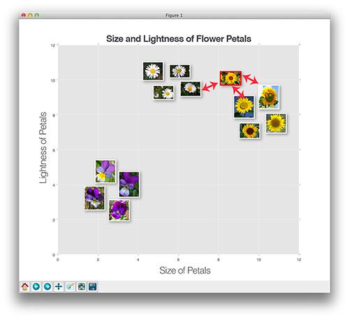
The k-Nearest Neighbors classifier is by far the most simple image classification algorithm.

In fact, it’s so simple that it doesn’t actually “learn” anything. Instead, this algorithm relies on the distance between feature vectors. Simply put, the k-NN algorithm classifies unknown data points by finding the most common class among the k closest examples.

Each data point in the k closest data points casts a vote and the category with the highest number of votes wins!

Or, in plain English: “Tell me who your neighbors are, and I’ll tell you who you are.”

For example, in Figure 6 above we see three sets of our flowers:

• Daises
• Pansies
• Sunflowers

We have plotted each of the flower images according to their lightness of the petals (color) and the size of the petals (this is an arbitrary example so excuse the non-formality).

We can clearly see that the image is a sunflower, but what does k-NN think given our new image is equal distance to one pansy and two sunflowers?

Well, k-NN would examine the three closest neighbors (k=3) and since there are two votes for sunflowers versus one vote for pansies, the sunflower class would be selected.

To put k-NN in action, make sure you’ve used the “Downloads” section of the tutorial to download the source code and example datasets.

From there, open up a terminal and execute the following command:

$ python classify_iris.py 
[INFO] loading data...
[INFO] using 'knn' model
[INFO] evaluating...
              precision    recall  f1-score   support

      setosa       1.00      1.00      1.00        15
  versicolor       0.92      0.92      0.92        12
   virginica       0.91      0.91      0.91        11

   micro avg       0.95      0.95      0.95        38
   macro avg       0.94      0.94      0.94        38

Here you can see that k-NN is obtaining 95% accuracy on the Iris dataset, not a bad start!

Let’s look at our 3-scenes dataset:

python classify_images.py --model knn
[INFO] extracting image features...
[INFO] using 'knn' model
[INFO] evaluating...
              precision    recall  f1-score   support

       coast       0.84      0.68      0.75       105
      forest       0.78      0.77      0.77        78
     highway       0.56      0.78      0.65        54

   micro avg       0.73      0.73      0.73       237
   macro avg       0.72      0.74      0.72       237
weighted avg       0.75      0.73      0.73       237

On the 3-scenes dataset, the k-NN algorithm is obtaining 75% accuracy.

In particular, k-NN is struggling to recognize the “highway” class (~56% accuracy).

We’ll be exploring methods to improve our image classification accuracy in the rest of this tutorial.

For more information on how the k-Nearest Neighbors algorithm works, be sure to refer to this post.

Naïve Bayes

After k-NN, Naïve Bayes is often the first true machine learning algorithm a practitioner will study.

The algorithm itself has been around since the 1950s and is often used to obtain baselines for future experiments (especially in domains related to text retrieval).

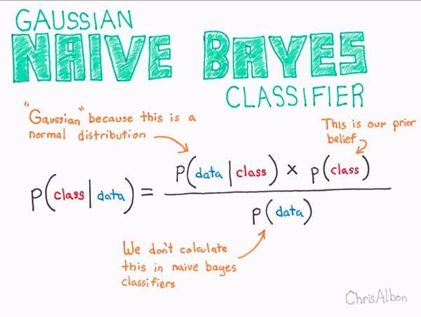
The Naïve Bayes algorithm is made possible due to Bayes’ theorem (Figure 7).

Essentially, Naïve Bayes formulates classification as an expected probability.

Given our input data, D, we seek to compute the probability of a given class, C.

Formally, this becomes P(C | D).

To actually compute the probability we compute the numerator of Figure 7 (ignoring the denominator).

The expression can be interpreted as:

1. Computing the probability of our input data given the class (ex., the probability of a given flower being Iris Setosa having a sepal length of 4.9cm)
2. Then multiplying by the probability of us encountering that class throughout the population of the data (ex. the probability of even encountering the Iris Setosa class in the first place)

Let’s go ahead and apply the Naïve Bayes algorithm to the Iris dataset:

$ python classify_iris.py --model naive_bayes
[INFO] loading data...
[INFO] using 'naive_bayes' model
[INFO] evaluating...
              precision    recall  f1-score   support

      setosa       1.00      1.00      1.00        15
  versicolor       1.00      0.92      0.96        12
   virginica       0.92      1.00      0.96        11

   micro avg       0.97      0.97      0.97        38
   macro avg       0.97      0.97      0.97        38
weighted avg       0.98      0.97      0.97        38

We are now up to 98% accuracy, a marked increase from the k-NN algorithm!

Now let’s apply Naïve Bayes to the 3-scenes dataset for image classification:

$ python classify_images.py --model naive_bayes
[INFO] extracting image features...
[INFO] using 'naive_bayes' model
[INFO] evaluating...
              precision    recall  f1-score   support

       coast       0.69      0.40      0.50        88
      forest       0.68      0.82      0.74        84
     highway       0.61      0.78      0.68        65

   micro avg       0.65      0.65      0.65       237
   macro avg       0.66      0.67      0.64       237
weighted avg       0.66      0.65      0.64       237

Uh oh!

It looks like we only obtained 66% accuracy here.

Does that mean that k-NN is better than Naïve Bayes and that we should always use k-NN for image classification?

Not so fast.

All we can say here is that for this particular project and for this particular set of extracted features the k-NN machine learning algorithm outperformed Naive Bayes.

We cannot say that k-NN is better than Naïve Bayes and that we should always use k-NN instead.

Thinking that one machine learning algorithm is always better than the other is a trap I see many new machine learning practitioners fall into — don’t make that mistake.

For more information on the Naïve Bayes machine learning algorithm, be sure to refer to this excellent article.

Logistic Regression

The next machine learning algorithm we are going to explore is Logistic Regression.

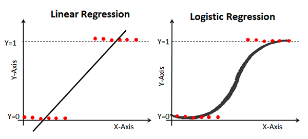
Logistic Regression is a supervised classification algorithm often used to predict the probability of a class label (the output of a Logistic Regression algorithm is always in the range [0, 1]).

Logistic Regression is heavily used in machine learning and is an algorithm any machine learning practitioner needs Logistic Regression in their Python toolbox.

Let’s apply Logistic Regression to the Iris dataset:

$ python classify_iris.py --model logit
[INFO] loading data...
[INFO] using 'logit' model
[INFO] evaluating...
              precision    recall  f1-score   support

      setosa       1.00      1.00      1.00        15
  versicolor       1.00      0.92      0.96        12
   virginica       0.92      1.00      0.96        11

   micro avg       0.97      0.97      0.97        38
   macro avg       0.97      0.97      0.97        38
weighted avg       0.98      0.97      0.97        38

Here we are able to obtain 98% classification accuracy!

And furthermore, note that both the Setosa and Versicolor classes are classified 100% correctly!

Now let’s apply Logistic Regression to the task of image classification:

$ python classify_images.py --model logit
[INFO] extracting image features...
[INFO] using 'logit' model
[INFO] evaluating...
              precision    recall  f1-score   support

       coast       0.67      0.67      0.67        92
      forest       0.79      0.82      0.80        82
     highway       0.61      0.57      0.59        63

   micro avg       0.70      0.70      0.70       237
   macro avg       0.69      0.69      0.69       237
weighted avg       0.69      0.70      0.69       237

Logistic Regression performs slightly better than Naive Bayes here, obtaining 69% accuracy but in order to beat k-NN we’ll need a more powerful Python machine learning algorithm.

Support Vector Machines (SVMs)

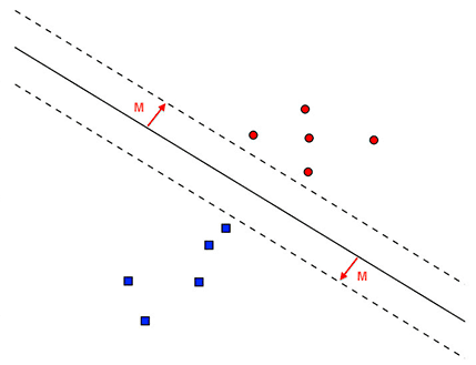
Support Vector Machines (SVMs) are extremely powerful machine learning algorithms capable of learning separating hyperplanes on non-linear datasets through the kernel trick.

If a set of data points are not linearly separable in an N-dimensional space we can project them to a higher dimension — and perhaps in this higher dimensional space the data points are linearly separable.

The problem with SVMs is that it can be a pain to tune the knobs on an SVM to get it to work properly, especially for a new Python machine learning practitioner.

When using SVMs it often takes many experiments with your dataset to determine:

1. The appropriate kernel type (linear, polynomial, radial basis function, etc.)
2. Any parameters to the kernel function (ex. degree of the polynomial)

If, at first, your SVM is not obtaining reasonable accuracy you’ll want to go back and tune the kernel and associated parameters — tuning those knobs of the SVM is critical to obtaining a good machine learning model. With that said, let’s apply an SVM to our Iris dataset:

$ python classify_iris.py --model svm
[INFO] loading data...
[INFO] using 'svm' model
[INFO] evaluating...
              precision    recall  f1-score   support

      setosa       1.00      1.00      1.00        15
  versicolor       1.00      0.92      0.96        12
   virginica       0.92      1.00      0.96        11

   micro avg       0.97      0.97      0.97        38
   macro avg       0.97      0.97      0.97        38
weighted avg       0.98      0.97      0.97        38

Just like Logistic Regression, our SVM obtains 98% accuracy — in order to obtain 100% accuracy on the Iris dataset with an SVM, we would need to further tune the parameters to the kernel.

Let’s apply our SVM to the 3-scenes dataset:

$ python classify_images.py --model svm
[INFO] extracting image features...
[INFO] using 'svm' model
[INFO] evaluating...
              precision    recall  f1-score   support

       coast       0.84      0.76      0.80        92
      forest       0.86      0.93      0.89        84
     highway       0.78      0.80      0.79        61

   micro avg       0.83      0.83      0.83       237
   macro avg       0.83      0.83      0.83       237

Wow, 83% accuracy!

That’s the best accuracy we’ve seen thus far!

Clearly, when tuned properly, SVMs lend themselves well to non-linearly separable datasets.

Decision Trees

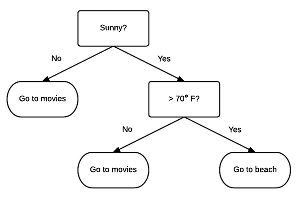
The basic idea behind a decision tree is to break classification down into a set of choices about each entry in our feature vector.

We start at the root of the tree and then progress down to the leaves where the actual classification is made.

Unlike many machine learning algorithms such which may appear as a “black box” learning algorithm (where the route to the decision can be hard to interpret and understand), decision trees can be quite intuitive — we can actually visualize and interpret the choice the tree is making and then follow the appropriate path to classification.

For example, let’s pretend we are going to the beach for our vacation. We wake up the first morning of our vacation and check the weather report — sunny and 90 degrees Fahrenheit.

That leaves us with a decision to make: “What should we do today? Go to the beach? Or see a movie?”

Subconsciously, we may solve the problem by constructing a decision tree of our own (Figure 10).

First, we need to know if it’s sunny outside.

A quick check of the weather app on our smartphone confirms that it is indeed sunny.

We then follow the Sunny=Yes branch and arrive at the next decision — is it warmer than 70 degrees out?

Again, after checking the weather app we can confirm that it will be > 70 degrees outside today.

Following the >70=Yes branch leads us to a leaf of the tree and the final decision — it looks like we are going to the beach!

Internally, decision trees examine our input data and look for the best possible nodes/values to split on using algorithms such as CART or ID3. The tree is then automatically built for us and we are able to make predictions.

Let’s go ahead and apply the decision tree algorithm to the Iris dataset:

$ python classify_iris.py --model decision_tree
[INFO] loading data...
[INFO] using 'decision_tree' model
[INFO] evaluating...
              precision    recall  f1-score   support

      setosa       1.00      1.00      1.00        15
  versicolor       0.92      0.92      0.92        12
   virginica       0.91      0.91      0.91        11

   micro avg       0.95      0.95      0.95        38
   macro avg       0.94      0.94      0.94        38
weighted avg       0.95      0.95      0.95        38

Our decision tree is able to obtain 95% accuracy.

What about our image classification project?

$ python classify_images.py --model decision_tree
[INFO] extracting image features...
[INFO] using 'decision_tree' model
[INFO] evaluating...
              precision    recall  f1-score   support

       coast       0.71      0.74      0.72        85
      forest       0.76      0.80      0.78        83
     highway       0.77      0.68      0.72        69

   micro avg       0.74      0.74      0.74       237
   macro avg       0.75      0.74      0.74       237
weighted avg       0.74      0.74      0.74       237

Here we obtain 74% accuracy — not the best but certainly not the worst either.

Random Forests

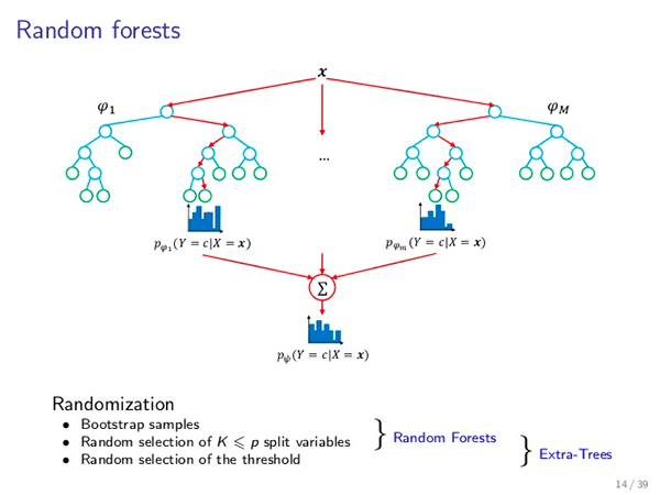
Since a forest is a collection of trees, a Random Forest is a collection of decision trees.

However, as the name suggestions, Random Forests inject a level of “randomness” that is not present in decision trees — this randomness is applied at two points in the algorithm.

• Bootstrapping — Random Forest classifiers train each individual decision tree on a bootstrapped sample from the original training data. Essentially, bootstrapping is sampling with replacement a total of D times. Bootstrapping is used to improve the accuracy of our machine learning algorithms while reducing the risk of overfitting.
• Randomness in node splits — For each decision tree a Random Forest trains, the Random Forest will only give the decision tree a portion of the possible features.

In practice, injecting randomness into the Random Forest classifier by bootstrapping training samples for each tree, followed by only allowing a subset of the features to be used for each tree, typically leads to a more accurate classifier.

At prediction time, each decision tree is queried and then the meta-Random Forest algorithm tabulates the final results.

Let’s try our Random Forest on the Iris dataset:

$ python classify_iris.py --model random_forest
[INFO] loading data...
[INFO] using 'random_forest' model
[INFO] evaluating...
              precision    recall  f1-score   support

      setosa       1.00      1.00      1.00        15
  versicolor       1.00      0.83      0.91        12
   virginica       0.85      1.00      0.92        11

   micro avg       0.95      0.95      0.95        38
   macro avg       0.95      0.94      0.94        38
weighted avg       0.96      0.95      0.95        38

As we can see, our Random Forest obtains 96% accuracy, slightly better than using just a single decision tree.

But what about for image classification?

Do Random Forests work well for our 3-scenes dataset?

$ python classify_images.py --model random_forest
[INFO] extracting image features...
[INFO] using 'random_forest' model
[INFO] evaluating...
              precision    recall  f1-score   support

       coast       0.80      0.83      0.81        84
      forest       0.92      0.84      0.88        90
     highway       0.77      0.81      0.79        63

   micro avg       0.83      0.83      0.83       237
   macro avg       0.83      0.83      0.83       237
weighted avg       0.84      0.83      0.83       237

Using a Random Forest we’re able to obtain 84% accuracy, a full 10% better than using just a decision tree.

In general, if you find that decision trees work well for your machine learning and Python project, you may want to try Random Forests as well!

Neural Networks

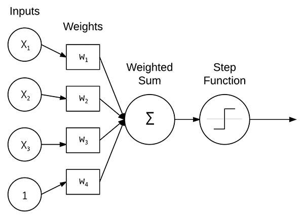
One of the most common neural network models is the Perceptron, a linear model used for classification.

A Perceptron accepts a set of inputs, takes the dot product between the inputs and the weights, computes a weighted sum, and then applies a step function to determine the output class label.

We typically don’t use the original formulation of Perceptrons as we now have more advanced machine learning and deep learning models. Furthermore, since the advent of the backpropagation algorithm, we can train multi-layer Perceptrons (MLP).

Combined with non-linear activation functions, MLPs can solve non-linearly separable datasets as well.

Let’s apply a Multi-layer Perceptron machine learning algorithm to our Iris dataset using Python and scikit-learn:

$ python classify_iris.py --model mlp
[INFO] loading data...
[INFO] using 'mlp' model
[INFO] evaluating...
              precision    recall  f1-score   support

      setosa       1.00      1.00      1.00        15
  versicolor       1.00      0.92      0.96        12
   virginica       0.92      1.00      0.96        11

   micro avg       0.97      0.97      0.97        38
   macro avg       0.97      0.97      0.97        38
weighted avg       0.98      0.97      0.97        38

Our MLP performs well here, obtaining 98% classification accuracy.

Let’s move on to image classification with an MLP:

$ python classify_images.py --model mlp
[INFO] extracting image features...
[INFO] using 'mlp' model
[INFO] evaluating...
              precision    recall  f1-score   support

       coast       0.72      0.91      0.80        86
      forest       0.92      0.89      0.90        79
     highway       0.79      0.58      0.67        72

   micro avg       0.80      0.80      0.80       237
   macro avg       0.81      0.79      0.79       237
weighted avg       0.81      0.80      0.80       237

The MLP reaches 81% accuracy here — quite respectable given the simplicity of the model!

Deep Learning and Deep Neural Networks

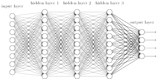
If you’re interested in machine learning and Python then you’ve likely encountered the term deep learning as well.

What exactly is deep learning?

And what makes it different than standard machine learning?

Well, to start, it’s first important to understand that deep learning is a subfield of machine learning, which is, in turn, a subfield of the larger Artificial Intelligence (AI) field.

The term “deep learning” comes from training neural networks with many hidden layers.

In fact, in the 1990s it was extremely challenging to train neural networks with more than two hidden layers due to (paraphrasing Geoff Hinton):

1. Our labeled datasets being too small
2. Our computers being far too slow
3. Not being able to properly initialize our neural network weights prior to training
4. Using the wrong type of nonlinearity function

It’s a different story now. We now have:

1. Faster computers
2. Highly optimized hardware (i.e., GPUs)
3. Large, labeled datasets
4. A better understanding of weight initialization
5. Superior activation functions

All of this has culminated at exactly the right time to give rise to the latest incarnation of deep learning.

And chances are, if you’re reading this tutorial on machine learning then you’re most likely interested in deep learning as well!

To gain some experience with neural networks, let’s implement one using Python and Keras.

Open up the nn_iris.py and insert the following code:

# import the necessary packages
from keras.models import Sequential
from keras.layers.core import Dense
from keras.optimizers import SGD
from sklearn.preprocessing import LabelBinarizer
from sklearn.model_selection import train_test_split
from sklearn.metrics import classification_report
from sklearn.datasets import load_iris

# load the Iris dataset and perform a training and testing split,
# using 75% of the data for training and 25% for evaluation
print("[INFO] loading data...")
dataset = load_iris()
(trainX, testX, trainY, testY) = train_test_split(dataset.data,
	dataset.target, test_size=0.25)

# encode the labels as 1-hot vectors
lb = LabelBinarizer()
trainY = lb.fit_transform(trainY)
testY = lb.transform(testY)

Let’s import our packages.

Our Keras imports are for creating and training our simple neural network (Lines 2-4). You should recognize the scikit-learn imports by this point (Lines 5-8).

We’ll go ahead and load + split our data and one-hot encode our labels on Lines 13-20. A one-hot encoded vector consists of binary elements where one of them is “hot” such as [0, 0, 1] or [1, 0, 0] in the case of our three flower classes.

Now let’s build our neural network:

# define the 4-3-3-3 architecture using Keras
model = Sequential()
model.add(Dense(3, input_shape=(4,), activation="sigmoid"))
model.add(Dense(3, activation="sigmoid"))
model.add(Dense(3, activation="softmax"))

Our neural network consists of two fully connected layers using sigmoid activation.

The final layer has a “softmax classifier” which essentially means that it has an output for each of our classes and the outputs are probability percentages.

Let’s go ahead and train and evaluate our model :

# train the model using SGD
print("[INFO] training network...")
opt = SGD(lr=0.1, momentum=0.9, decay=0.1 / 250)
model.compile(loss="categorical_crossentropy", optimizer=opt,
	metrics=["accuracy"])
H = model.fit(trainX, trainY, validation_data=(testX, testY),
	epochs=250, batch_size=16)

# evaluate the network
print("[INFO] evaluating network...")
predictions = model.predict(testX, batch_size=16)
print(classification_report(testY.argmax(axis=1),
	predictions.argmax(axis=1), target_names=dataset.target_names))

Our model is compiled on Lines 30-32 and then the training is initiated on Lines 33 and 34.

Just as with our previous two scripts, we’ll want to check on the performance by evaluating our network. This is accomplished by making predictions on our testing data and then printing a classification report (Lines 38-40).

There’s a lot going on under the hood in these short 40 lines of code. For an in-depth walkthrough of neural network fundamentals, please refer to the Starter Bundle of Deep Learning for Computer Vision with Python or the PyImageSearch Gurus course.

We’re down to the moment of truth — how will our neural network perform on the Iris dataset?

$ python nn_iris.py 
Using TensorFlow backend.
[INFO] loading data...
[INFO] training network...
Train on 112 samples, validate on 38 samples
Epoch 1/250
2019-01-04 10:28:19.104933: I tensorflow/core/platform/cpu_feature_guard.cc:141] Your CPU supports instructions that this TensorFlow binary was not compiled to use: AVX2 AVX512F FMA
112/112 [==============================] - 0s 2ms/step - loss: 1.1454 - acc: 0.3214 - val_loss: 1.1867 - val_acc: 0.2368
Epoch 2/250
112/112 [==============================] - 0s 48us/step - loss: 1.0828 - acc: 0.3929 - val_loss: 1.2132 - val_acc: 0.5000
Epoch 3/250
112/112 [==============================] - 0s 47us/step - loss: 1.0491 - acc: 0.5268 - val_loss: 1.0593 - val_acc: 0.4737
...
Epoch 248/250
112/112 [==============================] - 0s 46us/step - loss: 0.1319 - acc: 0.9554 - val_loss: 0.0407 - val_acc: 1.0000
Epoch 249/250
112/112 [==============================] - 0s 46us/step - loss: 0.1024 - acc: 0.9643 - val_loss: 0.1595 - val_acc: 0.8947
Epoch 250/250
112/112 [==============================] - 0s 47us/step - loss: 0.0795 - acc: 0.9821 - val_loss: 0.0335 - val_acc: 1.0000
[INFO] evaluating network...
             precision    recall  f1-score   support

     setosa       1.00      1.00      1.00         9
 versicolor       1.00      1.00      1.00        10
  virginica       1.00      1.00      1.00        19

avg / total       1.00      1.00      1.00        38

Wow, perfect! We hit 100% accuracy!

This neural network is the first Python machine learning algorithm we’ve applied that’s been able to hit 100% accuracy on the Iris dataset.

The reason our neural network performed well here is because we leveraged:

1. Multiple hidden layers
2. Non-linear activation functions (i.e., the sigmoid activation function)

Given that our neural network performed so well on the Iris dataset we should assume similar accuracy on the image dataset as well, right? Well, we actually have a trick up our sleeve — to obtain even higher accuracy on image datasets we can use a special type of neural network called a Convolutional Neural Network.

Convolutional Neural Networks

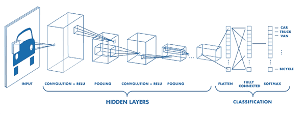
Convolutional Neural Networks, or CNNs for short, are special types of neural networks that lend themselves well to image understanding tasks. Unlike most machine learning algorithms, CNNs operate directly on the pixel intensities of our input image — no need to perform feature extraction!

Internally, each convolution layer in a CNN is learning a set of filters. These filters are convolved with our input images and patterns are automatically learned. We can also stack these convolution operates just like any other layer in a neural network.

Let’s go ahead and learn how to implement a simple CNN and apply it to basic image classification.

Open up the basic_cnn.py script and insert the following code:

# import the necessary packages
from keras.models import Sequential
from keras.layers.convolutional import Conv2D
from keras.layers.convolutional import MaxPooling2D
from keras.layers.core import Activation
from keras.layers.core import Flatten
from keras.layers.core import Dense
from keras.optimizers import Adam
from sklearn.preprocessing import LabelBinarizer
from sklearn.model_selection import train_test_split
from sklearn.metrics import classification_report
from PIL import Image
from imutils import paths
import numpy as np
import argparse
import os

# construct the argument parser and parse the arguments
ap = argparse.ArgumentParser()
ap.add_argument("-d", "--dataset", type=str, default="3scenes",
	help="path to directory containing the '3scenes' dataset")
args = vars(ap.parse_args())

In order to build a Convolutional Neural Network for machine learning with Python and Keras, we’ll need five additional Keras imports on Lines 2-8.

This time, we’re importing convolutional layer types, max pooling operations, different activation functions, and the ability to flatten. Additionally, we’re using the Adam optimizer rather than SGD as we did in the previous simple neural network script.

You should be acquainted with the names of the scikit-learn and other imports by this point.

This script has a single command line argument, --dataset . It represents the path to the 3-scenes directory on disk again.

Let’s load the data now:

# grab all image paths in the input dataset directory, then initialize
# our list of images and corresponding class labels
print("[INFO] loading images...")
imagePaths = paths.list_images(args["dataset"])
data = []
labels = []

# loop over our input images
for imagePath in imagePaths:
	# load the input image from disk, resize it to 32x32 pixels, scale
	# the pixel intensities to the range [0, 1], and then update our
	# images list
	image = Image.open(imagePath)
	image = np.array(image.resize((32, 32))) / 255.0
	data.append(image)

	# extract the class label from the file path and update the
	# labels list
	label = imagePath.split(os.path.sep)[-2]
	labels.append(label)

Similar to our classify_images.py script, we’ll go ahead and grab our imagePaths and build our data and labels lists.

There’s one caveat this time which you should not overlook:

We’re operating on the raw pixels themselves rather than a color statistics feature vector. Take the time to review classify_images.py once more and compare it to the lines of basic_cnn.py .

In order to operate on the raw pixel intensities, we go ahead and resize each image to 32×32 and scale to the range [0, 1] by dividing by 255.0 (the max value of a pixel) on Lines 36 and 37. Then we add the resized and scaled image to the data list (Line 38).

Let’s one-hot encode our labels and split our training/testing data:

# encode the labels, converting them from strings to integers
lb = LabelBinarizer()
labels = lb.fit_transform(labels)

# perform a training and testing split, using 75% of the data for
# training and 25% for evaluation
(trainX, testX, trainY, testY) = train_test_split(np.array(data),
	np.array(labels), test_size=0.25)

And then build our image classification CNN with Keras:

# define our Convolutional Neural Network architecture
model = Sequential()
model.add(Conv2D(8, (3, 3), padding="same", input_shape=(32, 32, 3)))
model.add(Activation("relu"))
model.add(MaxPooling2D(pool_size=(2, 2), strides=(2, 2)))
model.add(Conv2D(16, (3, 3), padding="same"))
model.add(Activation("relu"))
model.add(MaxPooling2D(pool_size=(2, 2), strides=(2, 2)))
model.add(Conv2D(32, (3, 3), padding="same"))
model.add(Activation("relu"))
model.add(MaxPooling2D(pool_size=(2, 2), strides=(2, 2)))
model.add(Flatten())
model.add(Dense(3))
model.add(Activation("softmax"))

On Lines 55-67, demonstrate an elementary CNN architecture. The specifics aren’t important right now, but if you’re curious, you should:

• Read my Keras Tutorial which will keep you get up to speed with Keras
• Read through my book Deep Learning for Computer Vision with Python, which includes super practical walkthrough and hands-on tutorials
• Go through my blog post on the Keras Conv2D parameters, including what each parameter does and when to utilize that specific parameter

Let’s go ahead and train + evaluate our CNN model:

# train the model using the Adam optimizer
print("[INFO] training network...")
opt = Adam(lr=1e-3, decay=1e-3 / 50)
model.compile(loss="categorical_crossentropy", optimizer=opt,
	metrics=["accuracy"])
H = model.fit(trainX, trainY, validation_data=(testX, testY),
	epochs=50, batch_size=32)

# evaluate the network
print("[INFO] evaluating network...")
predictions = model.predict(testX, batch_size=32)
print(classification_report(testY.argmax(axis=1),
	predictions.argmax(axis=1), target_names=lb.classes_))

Our model is trained and evaluated similarly to our previous script.

Let’s give our CNN a try, shall we?

$ python basic_cnn.py 
Using TensorFlow backend.
[INFO] loading images...
[INFO] training network...
Train on 711 samples, validate on 237 samples
Epoch 1/50
711/711 [==============================] - 0s 629us/step - loss: 1.0647 - acc: 0.4726 - val_loss: 0.9920 - val_acc: 0.5359
Epoch 2/50
711/711 [==============================] - 0s 313us/step - loss: 0.9200 - acc: 0.6188 - val_loss: 0.7778 - val_acc: 0.6624
Epoch 3/50
711/711 [==============================] - 0s 308us/step - loss: 0.6775 - acc: 0.7229 - val_loss: 0.5310 - val_acc: 0.7553
...
Epoch 48/50
711/711 [==============================] - 0s 307us/step - loss: 0.0627 - acc: 0.9887 - val_loss: 0.2426 - val_acc: 0.9283
Epoch 49/50
711/711 [==============================] - 0s 310us/step - loss: 0.0608 - acc: 0.9873 - val_loss: 0.2236 - val_acc: 0.9325
Epoch 50/50
711/711 [==============================] - 0s 307us/step - loss: 0.0587 - acc: 0.9887 - val_loss: 0.2525 - val_acc: 0.9114
[INFO] evaluating network...
             precision    recall  f1-score   support

      coast       0.85      0.96      0.90        85
     forest       0.99      0.94      0.97        88
    highway       0.91      0.80      0.85        64

avg / total       0.92      0.91      0.91       237

Using machine learning and our CNN we are able to obtain 92% accuracy, far better than any of the previous machine learning algorithms we’ve tried in this tutorial!

Clearly, CNNs lend themselves very well to image understanding problems.

What do our Python + Machine Learning results mean?

On the surface, you may be tempted to look at the results of this post and draw conclusions such as:

• “Logistic Regression performed poorly on image classification, I should never use Logistic Regression.”
• “k-NN did fairly well at image classification, I’ll always use k-NN!”

Be careful with those types of conclusions and keep in mind the 5-step machine learning process I detailed earlier in this post:

1. Examine your problem
2. Prepare your data (raw data, feature extraction, feature engineering, etc.)
3. Spot-check a set of algorithms
4. Examine your results
5. Double-down on the algorithms that worked best

Each and every problem you encounter is going to be different in some manner.

Over time, and through lots of hands-on practice and experience, you will gain a “sixth sense” as to what machine learning algorithms will work well in a given situation.

However, until you reach that point you need to start by applying various machine learning algorithms, examining what works, and re-doubling your efforts on the algorithms that showed potential.

No two problems will be the same and, in some situations, a machine learning algorithm you once thought was “poor” will actually end up performing quite well!

Summary

In this tutorial, you learned how to get started with machine learning and Python.

Specifically, you learned how to train a total of nine different machine learning algorithms:

1. k-Nearest Neighbors (k-NN)
2. Naive Bayes
3. Logistic Regression
4. Support Vector Machines (SVMs)
5. Decision Trees
6. Random Forests
7. Perceptrons
8. Multi-layer, feedforward neural networks
9. Convolutional Neural Networks

We then applied our set of machine learning algorithms to two different domains:

1. Numerical data classification via the Iris dataset
2. Image classification via the 3-scenes dataset

I would recommend you use the Python code and associated machine learning algorithms in this tutorial as a starting point for your own projects.

Finally, keep in mind our five-step process of approaching a machine learning problem with Python (you may even want to print out these steps and keep them next to you):

1. Examine your problem
2. Prepare your data (raw data, feature extraction, feature engineering, etc.)
3. Spot-check a set of algorithms
4. Examine your results
5. Double-down on the algorithms that worked best

By using the code in today’s post you will be able to get your start in machine learning with Python — enjoy it and if you want to continue your machine learning journey, be sure to check out the PyImageSearch Gurus course, as well as my book, Deep Learning for Computer Vision with Python, where I cover machine learning, deep learning, and computer vision in detail.

To download the source code this post, and be notified when future tutorials are published here on PyImageSearch, just enter your email address in the form below.