k-NN classifier for image classification

Now that we’ve had a taste of Deep Learning and Convolutional Neural Networks in last week’s blog post on LeNet, we’re going to take a step back and start to study machine learning in the context of image classification in more depth.

To start, we’ll reviewing the k-Nearest Neighbor (k-NN) classifier, arguably the most simple, easy to understand machine learning algorithm. In fact, k-NN is so simple that it doesn’t perform any “learning” at all!

In the remainder of this blog post, I’ll detail how the k-NN classifier works. We’ll then apply k-NN to the Kaggle Dogs vs. Cats dataset, a subset of the Asirra dataset from Microsoft.

The goal of the Dogs vs. Cats dataset, as the name suggests, is to classify whether a given image contains a dog or a cat. We’ll be using this dataset a lot in future blog posts (for reasons I’ll explain later in this tutorial), so make sure you take the time now to read through this post and familiarize yourself with the dataset.

All that said, let’s get started implementing k-NN for image classification to recognize dogs vs. cats in images!

k-NN classifier for image classification

After getting your first taste of Convolutional Neural Networks last week, you’re probably feeling like we’re taking a big step backward by discussing k-NN today.

What gives?

Well, here’s the deal.

I once wrote a (controversial) blog post on getting off the deep learning bandwagon and getting some perspective. Despite the antagonizing title, the overall theme of this post centered around various trends in machine learning history, such as Neural Networks (and how research in NNs almost died in the 70-80’s), Support Vector Machines, and Ensemble methods.

When each of these methods were introduced, researchers and practitioners were equipped with new, powerful techniques — in essence, they were given a hammer and every problem looked like a nail, when in reality, all they needed was a few simple turns of a phillips head to solve a particular the problem.

I have news for you: Deep learning is no different.

Go to the vast majority of popular machine learning and computer vision conferences and look at the recent list of publications. What is the overarching theme?

Deep learning.

Then, hop on large LinkedIn groups related to computer vision and machine learning. What are many people asking about?

How to apply deep learning to their datasets.

After that, go over to popular computer science sub-reddits such as /r/machinelearning. What tutorials are the most consistently upvoted?

You guessed it: deep learning.

Here’s the bottom line:

Yes, I will teach you about Deep Learning and Convolutional Neural Networks on this blog — but you’re damn-well going to understand that Deep Learning is just a TOOL, and like any other tool, there is a right and wrong time to use it.

Because of this, it’s important for us to understand the basics of machine learning before we progress too far. Over the next few weeks, I’ll be discussing the basics of machine learning and Neural Networks, eventually building up to Deep Learning (where you’ll be able to appreciate the inner-workings of these algorithms more).

Kaggle Dogs vs. Cats dataset

The Dogs vs. Cats dataset was actually part of a Kaggle challenge a few years back. The challenge itself was simple: given an image, predict whether it contained a dog or a cat:

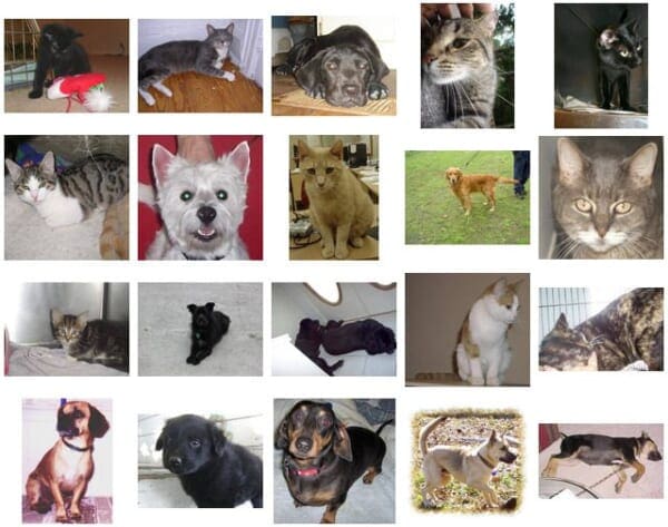
Simple enough — but if you know anything about image classification, you’ll understand that given:

• Viewpoint variation
• Scale variation
• Deformation
• Occlusion
• Background clutter
• Intra-class variation

That the problem is significantly harder than it might appear on the surface.

By simply randomly guessing, you should be able to reach 50% accuracy (since there are only two class labels). A machine learning algorithm will need to obtain > 50% accuracy in order to demonstrate that it has in fact “learned” something (or found an underlying pattern in the data).

Personally, I love the Dogs vs. Cats challenge, especially for teaching Deep Learning.

Why?

The dataset is simple enough to wrap your head around — there are only two classes: “dog” or “cat”.

However, the dataset is nicely sized, containing 25,000 images in the training data. This means that you have enough data to train data-hungry Convolutional Neural Networks from scratch.

We’ll be using this dataset a lot in future blog posts. I’ve actually included it in the “Downloads” section of this blog post for your convenience, so scroll down to grab the code + data before you follow along.

Project structure

Once you’ve downloaded the archive for this blog post, unzip it to someplace convenient. From there let’s take a look at the project directory structure:

$ tree --filelimit 10
.
├── kaggle_dogs_vs_cats
│   └── train [25000 entries exceeds filelimit, not opening dir]
└── knn_classifier.py

2 directories, 1 file

The Kaggle dataset is included in the kaggle_dogs_vs_cats/train directory (it comes from train.zip available on the Kaggle webpage).

We’ll be reviewing one Python script today — knn_classifier.py . This file will load the dataset, establish and run the K-NN classifier, and print out the evaluation metrics.

How does the k-NN classifier work?

The k-Nearest Neighbor classifier is by far the most simple machine learning/image classification algorithm. In fact, it’s so simple that it doesn’t actually “learn” anything.

Inside, this algorithm simply relies on the distance between feature vectors, much like building an image search engine — only this time, we have the labels associated with each image so we can predict and return an actual category for the image.

Simply put, the k-NN algorithm classifies unknown data points by finding the most common class among the k-closest examples. Each data point in the k closest examples casts a vote and the category with the most votes wins!

Or, in plain english: “Tell me who your neighbors are, and I’ll tell you who you are”

To visualize this, take a look at the following toy example where I have plotted the “fluffiness” of animals along the x-axis and the lightness of their coat on the y-axis:

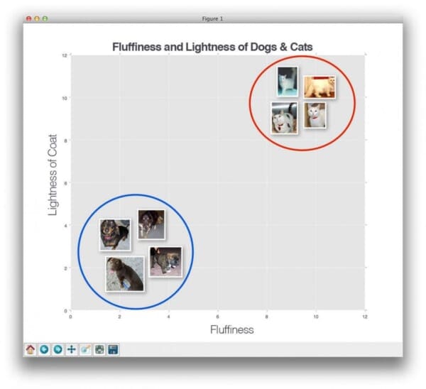
Here we can see there are two categories of images and that each of the data points within each respective category are grouped relatively close together in an n-dimensional space. Our dogs tend to have dark coats which are not very fluffy while our cats have very light coats that are extremely fluffy.

This implies that the distance between two data points in the red circle is much smaller than the distance between a data point in the red circle and a data point in the blue circle.

In order to apply the k-nearest Neighbor classification, we need to define a distance metric or similarity function. Common choices include the Euclidean distance:

And the Manhattan/city block distance:

Other distance metrics/similarity functions can be used depending on your type of data (the chi-squared distance is often used for distributions [i.e., histograms]). In today’s blog post, for the sake of simplicity, we’ll be using the Euclidean distance to compare images for similarity.

Implementing k-NN for image classification with Python

Now that we’ve discussed what the k-NN algorithm is, along with what dataset we’re going to apply it to, let’s write some code to actually perform image classification using k-NN.

Open up a new file, name it knn_classifier.py , and let’s get coding:

# import the necessary packages
from sklearn.neighbors import KNeighborsClassifier
from sklearn.model_selection import train_test_split
from imutils import paths
import numpy as np
import argparse
import imutils
import cv2
import os

We start off on Lines 2-9 by importing our required Python packages. If you haven’t already installed the scikit-learn library, then you’ll want to follow these instructions and install it now.

Note: This blog post has been updated to be compatible with the future scikit-learn==0.20 where sklearn.cross_validation has been replaced by sklearn.model_selection .

Secondly, we’ll be using the imutils library, a package that I have created to store common computer vision processing functions. If you do not have imutils installed, you’ll want to do that now:

$ pip install imutils

Next, we are going to define two methods to take an input image and convert it to a feature vector, or a list of numbers that quantify the contents of an image. The first method can be seen below:

def image_to_feature_vector(image, size=(32, 32)):
	# resize the image to a fixed size, then flatten the image into
	# a list of raw pixel intensities
	return cv2.resize(image, size).flatten()

The image_to_feature_vector method is an extremely naive function that simply takes an input image and resizes it to a fixed width and height (size ), and then flattens the RGB pixel intensities into a single list of numbers.

This means that our input image will be shrunk to 32 x 32 pixels, and given three channels for each Red, Green, and Blue component respectively, our output “feature vector” will be a list of 32 x 32 x 3 = 3,072 numbers.

Strictly speaking, the output of image_to_feature_vector is not a true “feature vector” since we tend to think of “features” and “descriptors” as abstract quantifications of the image contents.

Furthermore, utilizing raw pixel intensities as inputs to machine learning algorithms tends to yield poor results as even small changes in rotation, translation, viewpoint, scale, etc., can dramatically influence the image itself (and thus your output feature representation).

Note: As we’ll find out in later tutorials, Convolutional Neural Networks obtain fantastic results using raw pixel intensities as inputs — but this is because they learn a robust set of discriminating filters during the training process.

We then define our second method, this one called extract_color_histogram :

def extract_color_histogram(image, bins=(8, 8, 8)):
	# extract a 3D color histogram from the HSV color space using
	# the supplied number of `bins` per channel
	hsv = cv2.cvtColor(image, cv2.COLOR_BGR2HSV)
	hist = cv2.calcHist([hsv], [0, 1, 2], None, bins,
		[0, 180, 0, 256, 0, 256])

	# handle normalizing the histogram if we are using OpenCV 2.4.X
	if imutils.is_cv2():
		hist = cv2.normalize(hist)

	# otherwise, perform "in place" normalization in OpenCV 3 (I
	# personally hate the way this is done
	else:
		cv2.normalize(hist, hist)

	# return the flattened histogram as the feature vector
	return hist.flatten()

As the name suggests, this function accepts an input image and constructs a color histogram to characterize the color distribution of the image.

First, we convert our image to the HSV color space on Line 19. We then apply the cv2.calcHist function to compute a 3D color histogram for the image (Lines 20 and 21). You can read more about computing color histograms in this post. You might also be interested in applying color histograms to image search engines and in general, how to compate color histograms for similarity.

Given our computed hist , we then normalize it, taking care to use the appropriate cv2.normalize function signature based on our OpenCV version (Lines 24-30).

Given 8 bins for each of the Hue, Saturation, and Value channels respectively, our final feature vector is of size 8 x 8 x 8 = 512, thus our image is characterized by a 512-d feature vector.

Next, let’s parse our command line arguments:

# construct the argument parse and parse the arguments
ap = argparse.ArgumentParser()
ap.add_argument("-d", "--dataset", required=True,
	help="path to input dataset")
ap.add_argument("-k", "--neighbors", type=int, default=1,
	help="# of nearest neighbors for classification")
ap.add_argument("-j", "--jobs", type=int, default=-1,
	help="# of jobs for k-NN distance (-1 uses all available cores)")
args = vars(ap.parse_args())

We require only one command line argument, followed by two optional ones, each of which are detailed below:

• --dataset : This is the path to our input Kaggle Dogs vs. Cats dataset directory.
• --neighbors : Here we can supply the number of nearest neighbors that are taken into account when classifying a given data point. We’ll default this value to one, meaning that an image will be classified by finding its closest neighbor in an n–dimensional space and then taking the label of the closest image. In next week’s post, I’ll demonstrate how to automatically tune k for optimal accuracy.
• --jobs : Finding the nearest neighbor for a given image requires us to compute the distance from our input image to every other image in our dataset. This is clearly a O(N) operation that scales linearly. For larger datasets, this can become prohibitively slow. In order to speedup the process, we can distribute the computation of nearest neighbors across multiple processors/cores of our machine. Setting --jobs to -1 ensures that all processors/cores are used to help speedup the classification process.

Note: We can also speedup the k-NN classifier by utilizing specialized data structures such as kd-trees or Approximate Nearest Neighbor algorithms such as FLANN or Annoy. In practice, these algorithms can reduce nearest neighbor search to approximately O(log N); however, for the sake of simplicity in this post, we’ll perform an exhaustive nearest neighbor search.

We are now ready to prepare our images for feature extraction:

# grab the list of images that we'll be describing
print("[INFO] describing images...")
imagePaths = list(paths.list_images(args["dataset"]))

# initialize the raw pixel intensities matrix, the features matrix,
# and labels list
rawImages = []
features = []
labels = []

Line 47 grabs the paths to all 25,000 training images from disk.

We then initialize three lists (Lines 51-53) to store the raw image pixel intensities (the 3072-d feature vector), another to store the histogram features (the 512-d feature vector), and finally the class labels themselves (either “dog” or “cat”).

Let’s move on to extracting features from our dataset:

# loop over the input images
for (i, imagePath) in enumerate(imagePaths):
	# load the image and extract the class label (assuming that our
	# path as the format: /path/to/dataset/{class}.{image_num}.jpg
	image = cv2.imread(imagePath)
	label = imagePath.split(os.path.sep)[-1].split(".")[0]

	# extract raw pixel intensity "features", followed by a color
	# histogram to characterize the color distribution of the pixels
	# in the image
	pixels = image_to_feature_vector(image)
	hist = extract_color_histogram(image)

	# update the raw images, features, and labels matricies,
	# respectively
	rawImages.append(pixels)
	features.append(hist)
	labels.append(label)

	# show an update every 1,000 images
	if i > 0 and i % 1000 == 0:
		print("[INFO] processed {}/{}".format(i, len(imagePaths)))

We start looping over our input images on Line 56. Each image is loaded from disk and the class label is extracted from the imagePath (Lines 59 and 60).

We apply the image_to_feature_vector and extract_color_histogram functions on Lines 65 and 66 — these functions are used to extract our feature vectors from the input image .

Given our features labels, we then update the respective rawImages , features , and labels lists on Lines 70-72.

Finally, we display an update to our terminal to inform us on feature extraction progress every 1,000 images (Lines 75 and 76).

You might be curious how much memory our rawImages and features matrices take up — the following code block will tell us when executed:

# show some information on the memory consumed by the raw images
# matrix and features matrix
rawImages = np.array(rawImages)
features = np.array(features)
labels = np.array(labels)
print("[INFO] pixels matrix: {:.2f}MB".format(
	rawImages.nbytes / (1024 * 1000.0)))
print("[INFO] features matrix: {:.2f}MB".format(
	features.nbytes / (1024 * 1000.0)))

We start by converting our lists to NumPy arrays. We then use the .nbytes attribute of the NumPy array to display the number of megabytes of memory the representations utilize (about 75MB for the raw pixel intensities and 50MB for the color histograms. This implies that we can easily store our features in main memory).

Next, we need to take our data partition it into two splits — one for training and another for testing:

# partition the data into training and testing splits, using 75%
# of the data for training and the remaining 25% for testing
(trainRI, testRI, trainRL, testRL) = train_test_split(
	rawImages, labels, test_size=0.25, random_state=42)
(trainFeat, testFeat, trainLabels, testLabels) = train_test_split(
	features, labels, test_size=0.25, random_state=42)

Here we’ll be using 75% of our data for training and the remaining 25% for testing the k-NN algorithm.

Let’s apply the k-NN classifier to the raw pixel intensities:

# train and evaluate a k-NN classifer on the raw pixel intensities
print("[INFO] evaluating raw pixel accuracy...")
model = KNeighborsClassifier(n_neighbors=args["neighbors"],
	n_jobs=args["jobs"])
model.fit(trainRI, trainRL)
acc = model.score(testRI, testRL)
print("[INFO] raw pixel accuracy: {:.2f}%".format(acc * 100))

Here we instantiate the KNeighborsClassifier object from the scikit-learn library using the supplied number of --neighbors and --jobs .

We then “train” our model by making a call to .fit on Line 99, followed by evaluation on the testing data on Line 100.

In a similar fashion, we can also train and evaluate a k-NN classifier on our histogram representations:

# train and evaluate a k-NN classifer on the histogram
# representations
print("[INFO] evaluating histogram accuracy...")
model = KNeighborsClassifier(n_neighbors=args["neighbors"],
	n_jobs=args["jobs"])
model.fit(trainFeat, trainLabels)
acc = model.score(testFeat, testLabels)
print("[INFO] histogram accuracy: {:.2f}%".format(acc * 100))

k-NN image classification results

To test our k-NN image classifier, make sure you have downloaded the source code to this blog post using the “Downloads” form found at the bottom of this tutorial.

The Kaggle Dogs vs. Cats dataset is included with the download.

From there, just execute the following command:

$ python knn_classifier.py --dataset kaggle_dogs_vs_cats

At first, you’ll see that our images are being described and quantified via the image_to_feature_vector  and extract_color_histogram  functions:

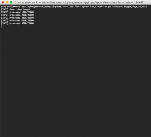
This process shouldn’t take longer than 1-3 minutes depending on the speed of your machine.

After the feature extraction process is complete, we can see some information on the size (in MB) of our feature representations:

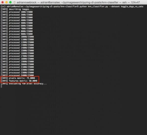
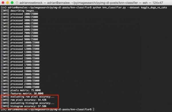
The raw pixel features take up 75MB while the color histograms require only 50MB of RAM.

Finally, the k-NN algorithm is trained and evaluated for both the raw pixel intensities and color histograms:

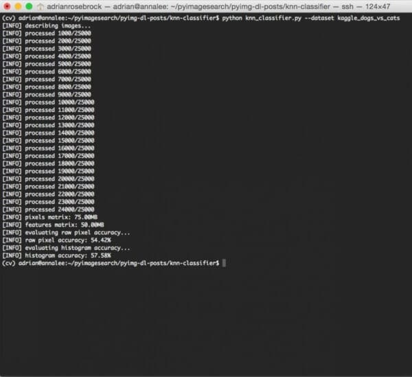
As the figure above demonstrates, by utilizing raw pixel intensities we were able to reach 54.42% accuracy. On the other hand, applying k-NN to color histograms achieved a slightly better 57.58% accuracy.

In both cases, we were able to obtain > 50% accuracy, demonstrating there is an underlying pattern to the images for both raw pixel intensities and color histograms.

However, that 57% accuracy leaves much to be desired.

And as you might imagine, color histograms aren’t the best way to distinguish between a dog and a cat:

• There are brown dogs. And there are brown cats.
• There are black dogs. And there are black cats.
• And certainly a dog and cat could appear in the same environment (such as a house, park, beach, etc.) where the background color distributions are similar.

Because of this, utilizing strictly color is not a great choice for characterizing the difference between dogs and cats — but that’s okay. The purpose of this blog post was simply to introduce the concept of image classification using the k-NN algorithm.

We can easily apply methods to obtain higher accuracy. And as we’ll see, utilizing Convolutional Neural Networks we can achieve > 95% accuracy without much effort — but I’ll save that for a future discussion once we better understand image classification.

Want to learn more about Convolutional Neural Networks right now?

If you enjoyed this tutorial on image classification, you’ll definitely want to take a look at the PyImageSearch Gurus course — the most complete, comprehensive computer vision course online today.

Inside the course, you’ll find over 168 lessons covering 2,161+ pages of content on Deep Learning, Convolutional Neural Networks, Image Classification, Face Recognition, and much more.

To learn more about the PyImageSearch Gurus course (and grab 10 FREE sample lessons + course syllabus), just click the button below:

 

Click here to learn more about PyImageSearch Gurus!

 

Can we do better?

You might be wondering, can we do better than the 57% classification accuracy?

You’ll notice that I’ve used only k=1 in this example, implying that only one nearest neighbor is considered when classifying each image. How would the results change if I used k=3 or k=5?

And how about the choice in distance metric — would the Manhattan/City block distance be a better choice?

How about changing both the value of k and distance metric at the same time?

Would classification accuracy improve? Get worse? Stay the same?

The fact is that nearly all machine learning algorithms require a bit of tuning to obtain optimal results. In order to determine the optimal set of values for these model variables, we apply a process called hyperparameter tuning, which is exactly the topic of next week’s blog post.

Summary

In this blog post, we reviewed the basics of image classification using the k-NN algorithm. We then applied the k-NN classifier to the Kaggle Dogs vs. Cats dataset to identify whether a given image contained a dog or a cat.

Utilizing only the raw pixel intensities of the input image images, we obtained 54.42% accuracy. And by using color histograms, we achieved a slightly better 57.58% accuracy. Since both of these results are > 50% (we should expect to get 50% accuracy simply by random guessing), we can ascertain that there is an underlying pattern in the raw pixels/color histograms that can be used to discriminate dogs vs. cats (although 57% accuracy is quite poor).

That raises the question: “Is it possible to obtain > 57% classification accuracy using k-NN? If so, how?”

The answer is hyperparameter tuning — which is exactly what we’ll be covering in next week’s blog post.

Be sure to sign up for the PyImageSearch Newsletter using the form below to be notified when the next blog post goes live!