Labeling superpixel colorfulness with OpenCV and Python

After our previous post on computing image colorfulness was published, Stephan, a PyImageSearch reader, left a comment on the tutorial asking if there was a method to compute the colorfulness of specific regions of an image (rather than the entire image).

There are multiple ways of attacking this problem. The first could be to apply a sliding window to loop over the image and compute the colorfulness score for each ROI. An image pyramid could even be applied if the colorfulness of a specific region needed to be computed at multiple scales.

However, a better approach would be to use superpixels. Superpixels are extracted via a segmentation algorithm that groups pixels into (non-rectangular) regions based on their local color/texture. In the case of the popular SLIC superpixel algorithm, image regions are grouped based on a local version of k-means clustering algorithm in the L*a*b* color space.

Given that superpixels will give us a much more natural segmentation of the input image than sliding windows, we can compute the colorfulness of specific regions in an image by:

1. Applying superpixel segmentation to the input image.
2. Looping over each of the superpixels individually and computing their respective colorfulness scores.
3. Maintaining a mask that contains the colorfulness score for each superpixel.

Based on this mask we can then visualize the most colorful regions of the image. Regions of the image that are more colorful will have larger colorful metric scores, while regions that are less colorful will smaller values.

To learn more about superpixels and computing image colorfulness, just keep reading.

Looking for the source code to this post?

Jump Right To The Downloads Section

Labeling superpixel colorfulness with OpenCV and Python

In the first part of this blog post we will learn how to apply the SLIC algorithm to extract superpixels from our input image. The original 2010 publication by Achanta et al., SLIC Superpixels, goes into the details of the methodology and technique. We also briefly covered SLIC superpixels in this blog post for readers who want a more concise overview of the algorithm.

Given these superpixels, we’ll loop over them individually and compute their colorfulness score, taking care to compute the colorfulness metric for the specific region and not the entire image (as we did in our previous post).

After we implement our script, we’ll apply our combination of superpixel + image colorfulness to a set of input images.

Using superpixels for segmentation

Let’s get started by opening up a new file in your favorite editor or IDE, name it colorful_regions.py , and insert the following code:

# import the necessary packages
from skimage.exposure import rescale_intensity
from skimage.segmentation import slic
from skimage.util import img_as_float
from skimage import io
import numpy as np
import argparse
import cv2

The first Lines 1-8 handle our imports — as you can see we make heavy use of several scikit-image functions in this tutorial.

The slic function will be used to compute superpixels (scikit-image documentation).

Next, we will define our colorfulness metric function with a minor modification from the previous post where it was introduced:

def segment_colorfulness(image, mask):
	# split the image into its respective RGB components, then mask
	# each of the individual RGB channels so we can compute
	# statistics only for the masked region
	(B, G, R) = cv2.split(image.astype("float"))
	R = np.ma.masked_array(R, mask=mask)
	G = np.ma.masked_array(B, mask=mask)
	B = np.ma.masked_array(B, mask=mask)

	# compute rg = R - G
	rg = np.absolute(R - G)

	# compute yb = 0.5 * (R + G) - B
	yb = np.absolute(0.5 * (R + G) - B)

	# compute the mean and standard deviation of both `rg` and `yb`,
	# then combine them
	stdRoot = np.sqrt((rg.std() ** 2) + (yb.std() ** 2))
	meanRoot = np.sqrt((rg.mean() ** 2) + (yb.mean() ** 2))

	# derive the "colorfulness" metric and return it
	return stdRoot + (0.3 * meanRoot)

Lines 10-31 represent our colorfulness metric function, which has been adapted to compute the colorfulness for a specific region of an image.

The region can be any shape as we take advantage of NumPy masked arrays — only pixels part of the mask will be included in the computation.

For the specified mask region of a particular image , the segment_colorfulness function performs the following tasks:

1. Splits the image into RGB component channels (Line 14).
2. Masks the image using mask (for each channel) so that the colorfulness is only performed on the area specified — in this case the region will be our superpixel (Lines 15-17).
3. Uses the R and G components to compute rg (Line 20).
4. Uses the RGB components to compute yb (Lines 23).
5. Computes the mean and standard deviation of rg and yb whilst combining them (Lines 27 and 28).
6. Does the final calculation of the metric and returns (Line 31) it to the calling function.

Now that our key colorfulness function is defined, the next step is to parse our command line arguments:

# construct the argument parse and parse the arguments
ap = argparse.ArgumentParser()
ap.add_argument("-i", "--image", required=True,
	help="path to input image")
ap.add_argument("-s", "--segments", type=int, default=100,
	help="# of superpixels")
args = vars(ap.parse_args())

On Lines 34-39 we make use of argparse to define two arguments:

1. --image : The path to our input image.
2. --segments : The number of superpixels. The SLIC Superpixels paper shows examples of breaking an image up into different numbers of superpixels. This parameter is fun to experiment with (as it controls the level of granularity of your resulting superpixels); however we’ll be working with a default=100 . The smaller the value, the fewer and larger the superpixels, allowing the algorithm running faster. The larger the number of segments, the more fine-grained the segmentation, but SLIC will take longer to run (due to more clusters needing to be computed).

Now it’s time to load the image into memory, allocate space for our visualization, and compute SLIC superpixel segmentation:

# load the image in OpenCV format so we can draw on it later, then
# allocate memory for the superpixel colorfulness visualization
orig = cv2.imread(args["image"])
vis = np.zeros(orig.shape[:2], dtype="float")

# load the image and apply SLIC superpixel segmentation to it via
# scikit-image
image = io.imread(args["image"])
segments = slic(img_as_float(image), n_segments=args["segments"],
	slic_zero=True)

On Line 43 we load our command line argument --image into memory as orig (OpenCV format).

We follow this step by allocating memory with the same shape (width and height) as the original input image for our visualization image, vis .

Next, we load the command line argument --image into memory as image , this time in scikit-image format. The reason we use scikit-image’s io.imread here is because OpenCV loads images in BGR order rather than RGB format (which scikit-image does). The slic function will convert our input image to the L*a*b* color space during the superpixel generation process assuming our image is in RGB format.

Therefore we have two choices:

1. Load the image with OpenCV, clone it, and then swap the ordering of the channels.
2. Simply load a copy of the original image using scikit-image.

Either approach is valid and will result in the same output.

Superpixels are calculated by a call to slic where we specify image , n_segments , and the slic_zero switch. Specifying slic_zero=True indicates that we want to use the zero parameter version of SLIC, an extension to the original algorithm that does not require us to manually tune parameters to the algorithm. We refer to the superpixels as segments for the rest of the script.

Now let’s compute the colorfulness of each superpixel:

# loop over each of the unique superpixels
for v in np.unique(segments):
	# construct a mask for the segment so we can compute image
	# statistics for *only* the masked region
	mask = np.ones(image.shape[:2])
	mask[segments == v] = 0

	# compute the superpixel colorfulness, then update the
	# visualization array
	C = segment_colorfulness(orig, mask)
	vis[segments == v] = C

We start by looping over each of the individual segments on Line 52.

Lines 56 and 57 are responsible for constructing a mask for the current superpixel. The mask will have the same width and height as our input image and will be filled (initially) with an array of ones (Line 56).

Keep in mind that when using NumPy masked arrays, that a given entry in an array is only included in a computation if the corresponding mask value is set to zero (implying that the pixel is unmasked). If the value in the mask is one, then the value is assumed to be masked and is hence ignored.

Here we initially set all pixels to masked, then set only the pixels part of the current superpixel to unmasked (Line 57).

Using our orig image and our mask as parameters to segment_colorfulness , we can compute C , which is the colorfulness of the superpixel (Line 61).

Then, we update our visualization array, vis , with the value of C (Line 62).

At this point, we have answered PyImageSearch reader, Stephan’s question — we have computed the colorfulness for different regions of an image.

Naturally we will want to see our results, so let’s continue by constructing a transparent overlay visualization for the most/least colorful regions in our input image:

# scale the visualization image from an unrestricted floating point
# to unsigned 8-bit integer array so we can use it with OpenCV and
# display it to our screen
vis = rescale_intensity(vis, out_range=(0, 255)).astype("uint8")

# overlay the superpixel colorfulness visualization on the original
# image
alpha = 0.6
overlay = np.dstack([vis] * 3)
output = orig.copy()
cv2.addWeighted(overlay, alpha, output, 1 - alpha, 0, output)

Since vis is currently a floating point array, it is necessary to re-scale it to a typical 8-bit unsigned integer [0-255] array. This is important so that we can display the output image to our screen with OpenCV. We accomplish this by using the rescale_intensity function (from skimage.exposure ) on Line 67.

Now we’ll overlay the superpixel colorfulness visualization on top of the original image. We’ve already discussed transparent overlays and the cv2.addWeighted (and associated parameters), so please refer to this blog post for more details on how transparent overlays are constructed.

Finally, let’s display images to the screen and close out this script:

# show the output images
cv2.imshow("Input", orig)
cv2.imshow("Visualization", vis)
cv2.imshow("Output", output)
cv2.waitKey(0)

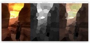
We will display three images to the screen using cv2.imshow , including:

1. orig : Our input image.
2. vis : Our visualization image (i.e., level of colorfulness for each of the superpixel regions).
3. output : Our output image.

Superpixel and colorfulness metric results

Let’s see our Python script in action — open a terminal, workon your virtual environment if you are using one (highly recommended), and enter the following command:

$ python colorful_regions.py --image images/example_01.jpg

On the left you can see the original input image, a photo of myself exploring Antelope Canyon, arguably the most beautiful slot canyon in the United States. Here we can see a mixture of colors due to the light filtering in from above.

In the middle we have our computed visualization for each of the 100 superpixels. Dark regions in this visualization refer to less colorful regions while light regions indicate more colorful.

Here we can see the least colorful regions are around the walls of the canyon, closest to the camera — this is where the least light is researching.

The most colorful regions of the input image are found where the light is directly reaching inside the canyon, illuminating part of the wall like candlelight.

Finally, on the right we have our original input image overlaid with the colorfulness visualization — this image allows us to more easily identify the most/least colorful regions of the image.

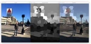
The following image is a photo of myself in Boston by the iconic Citgo sign overlooking Kenmore square:

$ python colorful_regions.py --image images/example_02.jpg

Here we can see the least colorful regions of the image are towards the bottom where the shadow is obscuring much of the sidewalk. The more colorful regions can be found towards the sign and sky itself.

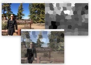
Finally, here is a photo from Rainbow Point, the highest elevation in Bryce Canyon:

$ python colorful_regions.py --image images/example_03.jpg

Notice here that my black hoodie and shorts are the least colorful regions of the image, while the sky and foliage towards the center of the photo are the most colorful.

What's next? We recommend PyImageSearch University.

Course information:
86 total classes • 115+ hours of on-demand code walkthrough videos • Last updated: October 2024
★★★★★ 4.84 (128 Ratings) • 16,000+ Students Enrolled

I strongly believe that if you had the right teacher you could master computer vision and deep learning.

Do you think learning computer vision and deep learning has to be time-consuming, overwhelming, and complicated? Or has to involve complex mathematics and equations? Or requires a degree in computer science?

That’s not the case.

All you need to master computer vision and deep learning is for someone to explain things to you in simple, intuitive terms. And that’s exactly what I do. My mission is to change education and how complex Artificial Intelligence topics are taught.

If you're serious about learning computer vision, your next stop should be PyImageSearch University, the most comprehensive computer vision, deep learning, and OpenCV course online today. Here you’ll learn how to successfully and confidently apply computer vision to your work, research, and projects. Join me in computer vision mastery.

Inside PyImageSearch University you'll find:

• ✓ 86 courses on essential computer vision, deep learning, and OpenCV topics
• ✓ 86 Certificates of Completion
• ✓ 115+ hours of on-demand video
• ✓ Brand new courses released regularly, ensuring you can keep up with state-of-the-art techniques
• ✓ Pre-configured Jupyter Notebooks in Google Colab
• ✓ Run all code examples in your web browser — works on Windows, macOS, and Linux (no dev environment configuration required!)
• ✓ Access to centralized code repos for all 540+ tutorials on PyImageSearch
• ✓ Easy one-click downloads for code, datasets, pre-trained models, etc.
• ✓ Access on mobile, laptop, desktop, etc.

Click here to join PyImageSearch University

Summary

In today’s blog post we learned how to use the SLIC segmentation algorithm to compute superpixels for an input image.

We then accessed each of the individual superpixels and applied our colorfulness metric.

The colorfulness scores for each region were combined into a mask, revealing the most colorful and least colorful regions of the input image.

Given this computation, we were able to visualize the colorfulness of each region in two ways:

1. By examining the raw vis mask.
2. Creating a transparent overlay that laid vis on top of the original image.

In practice, we could use this technique to threshold the mask and extract only the most/least colorful regions.

To be notified when future tutorials are published here on PyImageSearch, be sure to enter your email address in the form below!

Download the Source Code and FREE 17-page Resource Guide

Enter your email address below to get a .zip of the code and a FREE 17-page Resource Guide on Computer Vision, OpenCV, and Deep Learning. Inside you'll find my hand-picked tutorials, books, courses, and libraries to help you master CV and DL!

Download the code!

Website