Training with PyTorch Lightning: Structured MLOps Development

---

Training with PyTorch Lightning: Structured MLOps Development

In this lesson, you will learn how to build a fully modular, reproducible, and production-friendly training pipeline using PyTorch Lightning and Hydra. We will train a sentiment-classification model with a clean MLOps-ready structure that scales as your projects grow.

This lesson is the 1st in a 2-part series on PyTorch Lightning:

1. Training with PyTorch Lightning: Structured MLOps Development (this tutorial)
2. Lesson 2

To learn how to structure deep learning code for reliable, maintainable training workflows, just keep reading.

---

Why PyTorch Lightning Improves Reproducible MLOps Training Pipelines

Deep learning projects begin as small experiments (e.g., a single script, a few functions, and a quick training loop). But as your model grows, your dataset expands, and your experimentation increases, that simple script becomes a bottleneck. It collects data loading, model code, training logic, metrics, logging, and CLI arguments all in one place. This makes the code harder to debug, harder to reproduce, and nearly impossible to scale.

From an MLOps perspective, this is a critical issue. Reproducibility, modularity, logging, version control, and collaboration all depend on a clean separation of concerns. When data, modeling, and training logic live inside one file, versioning becomes fragile. Dockerization becomes harder. Running distributed or mixed-precision training becomes messy. And experiment tracking ends up inconsistent.

This is exactly where PyTorch Lightning shines. Instead of mixing everything together, Lightning organizes your training workflow into well-defined components:

• LightningModule: contains your model and training/validation/test logic
• LightningDataModule: manages data downloading, tokenization, and data loaders
• Trainer: handles the engineering: GPUs, mixed precision, checkpointing, logging, and training loops

You keep your PyTorch code. Lightning handles the boilerplate.

This separation is not just “clean code.” It is an MLOps superpower. With structure in place, you can:

• Version your data, model code, and configs separately
• Run consistent experiments across environments
• Scale from CPU → single GPU → multi-GPU → multi-node without changing code
• Produce reproducible artifacts for DVC and deployment
• Integrate Hydra configs for repeatable pipelines

In this lesson, you will see how Lightning transforms a typical sentiment-classification workflow into a modular, reproducible, production-ready training pipeline (i.e., the kind expected in real-world MLOps and LLMOps teams).

To learn how to structure reproducible ML training with PyTorch Lightning, just keep reading.

---

Would you like immediate access to 3,457 images curated and labeled with hand gestures to train, explore, and experiment with … for free? Head over to Roboflow and get a free account to grab these hand gesture images.

---

Configuring Your Development Environment

Before we begin implementing the training pipeline, let’s configure the development environment. This project uses modern versions of PyTorch, PyTorch Lightning, and the Hugging Face ecosystem, along with Hydra for configuration management. Installing the correct dependencies ensures that your training, data loading, and model export workflows run smoothly.

All the required libraries are pip-installable. Below is the full list of dependencies used in this lesson:

# PyTorch and Lightning
torch>=2.1.0
torchvision>=0.16.0
torchaudio>=2.1.0
pytorch-lightning>=2.1.0

# Hugging Face ecosystem
transformers>=4.35.0
datasets>=2.14.0
tokenizers>=0.15.0

# Configuration management
hydra-core>=1.3.0
omegaconf>=2.3.0

# Metrics and monitoring
torchmetrics>=1.2.0
tensorboard>=2.15.0

# Data processing
numpy>=1.24.0
pandas>=2.0.0

# Utilities
tqdm>=4.66.0
pyyaml>=6.0.0

You can install everything with a single command:

!pip install -r requirements.txt

Your project folder includes a requirements.txt file containing all of the dependencies above. If you are working inside a clean virtual environment (e.g., venv or Conda), this setup will give you everything needed to train the sentiment-classification model in Lesson 1.

---

Need Help Configuring Your Development Environment?

All that said, are you:

• Short on time?
• Learning on your employer’s administratively locked system?
• Wanting to skip the hassle of fighting with the command line, package managers, and virtual environments?
• Ready to run the code immediately on your Windows, macOS, or Linux system?

Then join PyImageSearch University today!

Gain access to Jupyter Notebooks for this tutorial and other PyImageSearch guides pre-configured to run on Google Colab’s ecosystem right in your web browser! No installation required.

And best of all, these Jupyter Notebooks will run on Windows, macOS, and Linux!

---

Project Structure

Before we write any code, it is important to understand how a real MLOps-ready training workflow is organized. A clean project structure makes your training pipeline easier to maintain, debug, scale across machines, and integrate later with DVC, MLflow, and CI/CD. PyTorch Lightning encourages this modular layout (e.g., through structured components), and Hydra takes care of configuration management in a clean, reproducible way.

Below is the project structure we will use for Lesson 1:

lesson1/
├── configs/
│   ├── config.yaml
│   ├── model/
│   │   └── distilbert.yaml
│   ├── data/
│   │   └── imdb.yaml
│   └── trainer/
│       └── default.yaml
└── src/
    ├── data_module.py
    ├── model_module.py
    ├── train.py
    └── inference.py

The src/ folder contains all the Python logic:

• data_module.py: handles dataset loading, tokenization, and data loaders
• model_module.py: defines the DistilBERT-based classifier
• train.py: orchestrates the training loop using PyTorch Lightning
• inference.py: allows you to test the trained model interactively

The configs/ directory is where we store all configuration files, grouped by purpose (model, data, trainer). This keeps hyperparameters and training settings cleanly separated from code, which is a fundamental principle in MLOps.

Hydra in 60 Seconds (All You Need for This Lesson)

Hydra is a configuration framework from Facebook Research that lets us manage all training settings (e.g., model hyperparameters, data parameters, and trainer options) in clean, reusable YAML files. Instead of hard-coding values inside Python, Hydra loads these configs automatically and lets you override anything from the command line.

This makes your training pipeline more reproducible, easier to maintain, and far more MLOps-friendly.

For example, you can change batch size, learning rate, or precision without editing the code:

python src/train.py data.batch_size=16 model.lr=3e-5 trainer.precision=16-mixed

Hydra merges the YAML configs at runtime (using config.yaml as the root), giving us a clean and scalable way to manage experiments.

Now that we understand how the project is organized and how Hydra helps us control training behavior, let us implement the LightningDataModule and build the first part of our training pipeline.

---

PyTorch LightningDataModule Explained: Building Efficient Data Pipelines

The LightningDataModule is one of the most important building blocks in PyTorch Lightning. It packages every data-related responsibility (e.g., downloading, preprocessing, tokenizing, and creating data loaders) into a single reusable module. This keeps your training loop clean and preserves a sharp separation between data code and model code, which is essential in any production-ready MLOps workflow.

In sentiment classification, the DataModule encapsulates 3 main tasks:

• loading the IMDB dataset: from Hugging Face
• tokenizing text: using a pretrained Transformer tokenizer
• producing data loaders: for train, validation, and test splits

Let us walk through the implementation step-by-step.

Before we start examining the class, let us begin with the imports that power this component of the pipeline:

import pytorch_lightning as pl
from datasets import load_dataset
from torch.utils.data import DataLoader
from transformers import AutoTokenizer

These 4 imports define everything the DataModule needs. pytorch_lightning gives us the LightningDataModule base class, which enforces a structured, reproducible way to manage data. load_dataset from Hugging Face handles downloading and preparing the IMDB dataset.

PyTorch’s DataLoader will assemble batches and handle multiprocessing, and AutoTokenizer loads the correct tokenizer for whichever transformer model we choose in the configuration.

Now that the foundations are clear, let us walk through the class itself.

Initializing the DataModule (__init__)

The constructor sets up every configurable part of the data pipeline.

Here is the code block we are examining:

class SentimentDataModule(pl.LightningDataModule):
    def __init__(
        self,
        model_name: str = "distilbert-base-uncased",
        dataset_name: str = "imdb",
        max_length: int = 128,
        batch_size: int = 8,
        num_workers: int = 4,
        **kwargs
    ):
        super().__init__()
        self.save_hyperparameters()
        
        self.model_name = model_name
        self.dataset_name = dataset_name
        self.max_length = max_length
        self.batch_size = batch_size
        self.num_workers = num_workers
        
        self.tokenizer = None
        self.train_dataset = None
        self.val_dataset = None
        self.test_dataset = None

The class inherits from pl.LightningDataModule, which means Lightning expects this object to implement the standard methods (prepare_data, setup, and the data loaders). The constructor receives all runtime-configurable parameters (e.g., which model tokenizer to use, which dataset to load, how long sequences should be, and what batch size to apply). These values are stored as instance attributes, but they are also captured automatically through self.save_hyperparameters(), enabling 2 important MLOps behaviors: experiment reproducibility and checkpoint metadata tracking.

The module initializes empty placeholders for the tokenizer and each dataset split. Nothing is loaded at this point. This keeps initialization fast, makes the DataModule safe for multiprocessing, and follows Lightning’s recommended pattern where all heavyweight work happens in the next 2 methods: prepare_data() and setup().

prepare_data(): One-Time Download Step

Next is the method prepare_data() that Lightning calls exactly once on a single process:

The constructor receives all hyperparameters needed to configure data preprocessing. Hydra will pass these values at runtime.

def prepare_data(self):
    load_dataset(self.dataset_name)
    AutoTokenizer.from_pretrained(self.model_name)

prepare_data() is responsible only for downloading the dataset and the tokenizer files. It does not tokenize or process anything; that comes later. The logic here intentionally has no side effects and does not assign anything to self. Lightning enforces this behavior because, in distributed training, only one GPU should perform downloads, while every GPU should independently run tokenization and data setup.

This separation is crucial for large-scale MLOps workflows because it prevents race conditions, avoids repetitive downloads, and maintains determinism across runs regardless of device or environment.

The setup() Method: Tokenization and Dataset Preparation

After the one-time download step in prepare_data(), Lightning calls the setup() method on every GPU (or CPU worker) participating in training. This is where the real work happens: tokenization, dataset formatting, and creating the train/validation/test splits. Because each device executes this method independently, the logic inside must be deterministic and side-effect-free, which is a core requirement when building reproducible training pipelines in distributed environments.

Here is the method we are explaining:

def setup(self, stage=None):
    self.tokenizer = AutoTokenizer.from_pretrained(self.model_name)
    
    if stage == "fit" or stage is None:
        dataset = load_dataset(self.dataset_name)

        self.train_dataset = dataset["train"].map(
            self._tokenize_function,
            batched=True,
            remove_columns=dataset["train"].column_names,
            desc="Tokenizing train set"
        )
        self.train_dataset.set_format("torch")

        self.val_dataset = dataset["test"].map(
            self._tokenize_function,
            batched=True,
            remove_columns=dataset["test"].column_names,
            desc="Tokenizing validation set"
        )
        self.val_dataset.set_format("torch")
    
    if stage == "test" or stage is None:
        dataset = load_dataset(self.dataset_name)
        self.test_dataset = dataset["test"].map(
            self._tokenize_function,
            batched=True,
            remove_columns=dataset["test"].column_names,
            desc="Tokenizing test set"
        )
        self.test_dataset.set_format("torch")

The first line initializes a fresh tokenizer instance. Lightning may spawn multiple processes in Distributed Data Parallel (DDP) or Fully Sharded Data Parallel (FSDP) mode, so each process needs its own tokenizer object. Tokenizers are stateless, lightweight, and safe to re-create, making them ideal for device-local initialization.

Lightning passes a stage identifier depending on what it is doing:

• fit: when calling trainer.fit()
• validate: when calling trainer.validate()
• test: when calling trainer.test()
• predict: when calling trainer.predict()
• None: Lightning did not specify a stage (certain internal flows)

Handling the None stage ensures the DataModule works correctly in all cases.

Inside the fit stage, we load the Hugging Face dataset. IMDB contains only train and test splits. Since it does not ship with an official validation set, this lesson uses the test split as validation. (In a real production MLOps pipeline, you would do a train/validation split yourself. This note will be added in the blog.)

Next comes tokenization. Hugging Face Datasets operates like a high-performance dataframe.

.map() applies _tokenize_function to every example or batch, efficiently processing the dataset:

• processes data in batches automatically
• parallelizes when possible
• avoids loading everything into memory

This is far more efficient and cleaner than writing custom loops.

After tokenization, we call self.train_dataset.set_format("torch"). This converts the dataset to output:

• torch.Tensor for inputs
• torch.Tensor for labels

which is exactly what PyTorch Lightning and the data loader expect. A nearly identical process prepares the validation dataset.

The test stage works the same way. Lightning may call fit and test separately, so we load and tokenize test data inside its own conditional block.

The logic inside setup() must be safe to run:

• once per GPU
• once per CPU worker
• once per stage

This is why nothing is written to disk or downloaded in this method. Everything is device-local: load → tokenize → return.

This is essential for:

• reproducibility
• distributed training
• multi-node training
• deterministic behavior in automated pipelines

Tokenization Logic: The Heart of Text Preprocessing

Tokenization is the most important preprocessing step in any natural language processing (NLP) pipeline. It converts raw text into numerical tensors that a Transformer model like DistilBERT can understand. Unlike image data (where pixel arrays are already numeric), text needs to be transformed from variable-length strings into fixed-length integer sequences.

In our DataModule, all tokenization runs through a single helper method:

def _tokenize_function(self, examples):
    tokenized = self.tokenizer(
        examples["text"],
        truncation=True,
        padding="max_length",
        max_length=self.max_length,
    )
    tokenized["labels"] = examples["label"]
    return tokenized

Let us break this down step-by-step.

The _tokenize_function handles the core preprocessing step for every text sample in the dataset. Hugging Face Datasets calls this function in batched mode, so examples["text"] is a list of movie reviews rather than a single string. The tokenizer processes the entire batch at once, which is significantly faster than looping over rows individually and also plays nicely with multiprocessing when multiple workers are specified in the data loader.

Inside the tokenizer call, we enable truncation and padding to a fixed max_length. Truncation ensures that very long reviews do not exceed the model’s maximum input window, keeping GPU memory usage predictable. Padding ensures that shorter reviews still produce fixed-length tensors, which is not only important for creating uniform batches but also becomes essential later when exporting the model to ONNX or TorchScript in Lesson 2 because both formats expect consistent input shapes.

After tokenization, we attach the corresponding labels by copying examples["label"] into the labels field. Hugging Face models expect this exact key during the forward pass when computing classification loss. This small remapping keeps the training step clean because the LightningModule can simply read batch["labels"] without any additional preprocessing or renaming logic.

The method finally returns a dictionary containing input_ids, attention_mask, and labels. Lightning and Hugging Face Datasets take care of converting these into PyTorch tensors later when we call .set_format("torch") in the setup() method. This tokenization pattern is highly scalable because it supports parallel CPU tokenization, remains deterministic for reproducibility, and works seamlessly in multi-GPU environments like DDP or FSDP. It is the same preprocessing approach used in large-scale NLP pipelines, from academic benchmarks to production systems handling millions of records.

Why This Approach Scales Well (MLOps Insight)

A major advantage of this design is how well it scales in real-world MLOps environments. Because _tokenize_function is used together with the Hugging Face .map() API, tokenization automatically runs in parallel across CPU workers. This gives you high throughput even when preprocessing millions of text samples. More importantly, the transformation is deterministic (the same input will always produce the same tokenized output), which is critical when you need reproducibility across training runs, machines, or distributed setups.

This pattern also integrates cleanly with multi-GPU training strategies (e.g., DDP and FSDP). Each GPU receives its own shard of the dataset and applies the exact same preprocessing logic, avoiding subtle mismatches between processes. Memory usage stays efficient as well, because batches are generated lazily and only the final tensorized output is kept in memory.

Finally, centralizing all preprocessing logic inside a single helper function makes the pipeline easy to maintain. Whether you’re training on a single GPU, scaling out to multiple nodes, or running the same preprocessing for offline batch inference, this structure remains robust. It’s the same approach used in production NLP systems where datasets can reach tens of millions of records and preprocessing needs to remain both fast and reliable.

Data Loaders: Batching Data for Training, Validation, and Testing

Once the dataset has been downloaded, tokenized, and formatted as tensors, the final component of the DataModule is producing PyTorch data loaders. These data loaders handle shuffling, batching, multiprocessing, and memory pinning, which are all needed to efficiently feed data into the model during training.

Here are the 3 data loader methods in our DataModule:

def train_dataloader(self):
    return DataLoader(
        self.train_dataset,
        batch_size=self.batch_size,
        shuffle=True,
        num_workers=self.num_workers,
        pin_memory=True
    )

def val_dataloader(self):
    return DataLoader(
        self.val_dataset,
        batch_size=self.batch_size,
        shuffle=False,
        num_workers=self.num_workers,
        pin_memory=True
    )

def test_dataloader(self):
    return DataLoader(
        self.test_dataset,
        batch_size=self.batch_size,
        shuffle=False,
        num_workers=self.num_workers,
        pin_memory=True
    )

Let us walk through these line-by-line.

The final part of the DataModule defines the 3 data loaders Lightning will use for training, validation, and testing. Each method returns a standard PyTorch DataLoader, but Lightning wires them together automatically inside trainer.fit(), so you do not need to manually pass datasets around.

The train_dataloader() creates batches from the tokenized training set and enables shuffle=True. Shuffling is essential for training stability because it prevents the model from seeing samples in the same order every epoch, which helps it generalize better. The batch size and number of workers come directly from the DataModule’s configuration, allowing Hydra to control them externally.

The val_dataloader() follows the same structure, except it disables shuffling. Validation should always process data in a fixed order because we want deterministic metrics that reflect model performance, not random input order.

Finally, the test_dataloader() mirrors the validation setup (no shuffling and the same batching logic), ensuring that evaluation on the test set is consistent and repeatable.

All 3 data loaders also set pin_memory=True, a small but meaningful performance optimization. When using GPUs, pinned memory allows faster host-to-device transfers, reducing input bottlenecks during training. Lightning will automatically handle device placement of data, so the data loaders simply provide ready-to-consume batches.

Overall, these 3 methods complete the DataModule’s lifecycle: downloading, tokenizing, splitting, and packaging the data into efficient data loaders. With these in place, the Trainer can run end-to-end training without any additional data plumbing from your side, which provides exactly the modularity and cleanliness we want in an MLOps-focused codebase.

Why This Loader Setup Works Well for MLOps

This pattern brings several production advantages:

• Works seamlessly with DDP/FSDP across multiple GPUs: Lightning automatically replicates data loaders across processes
• Fully deterministic: Regenerating the same batches across runs supports experiment reproducibility
• Fast I/O due to multiprocessing + pinned memory: Critical for high-speed training workloads
• Clear boundaries for debugging: If a batch is wrong, you know the issue is in the DataModule, not the model

---

PyTorch LightningModule Explained: Building Modular Deep Learning Models

The LightningModule is the heart of the training pipeline.

While the DataModule organizes data, the LightningModule organizes learning (the model architecture, forward pass, loss computation, metrics, and optimization strategy).

In plain terms, the LightningModule is where “what the model is” and “how the model learns” are defined.

For sentiment classification, the module wraps a pretrained DistilBERT encoder, adds a small classification head, and implements the training/validation/test logic needed for stable and reproducible NLP experiments.

Initialization: Building the Model Architecture

class SentimentClassifier(pl.LightningModule):
    def __init__(
        self,
        model_name: str = "distilbert-base-uncased",
        num_labels: int = 2,
        dropout: float = 0.1,
        lr: float = 2e-5,
        weight_decay: float = 0.01,
        **kwargs
    ):
        super().__init__()
        self.save_hyperparameters()

        config = AutoConfig.from_pretrained(model_name)
        self.encoder = AutoModel.from_pretrained(model_name, config=config)

        self.dropout = nn.Dropout(dropout)
        self.classifier = nn.Linear(config.hidden_size, num_labels)

        self.criterion = nn.CrossEntropyLoss()

        self.train_acc = Accuracy(task="multiclass", num_classes=num_labels)
        self.val_acc = Accuracy(task="multiclass", num_classes=num_labels)
        self.val_f1 = F1Score(task="multiclass", num_classes=num_labels, average="macro")

The constructor defines the core architecture and all hyperparameters needed for training. The use of self.save_hyperparameters() ensures that every setting (from model name to learning rate) is automatically captured in Lightning’s checkpoint files. This is extremely valuable in MLOps workflows because it makes every experiment self-describing and fully reproducible.

A DistilBERT encoder is loaded using the Hugging Face AutoModel, which instantly gives the model robust language understanding without any manual feature engineering. On top of that encoder, the model adds a simple dropout layer for regularization and a linear classifier to convert the encoded representation into sentiment logits. This small, clean architecture keeps training fast while still benefiting from the power of modern transformers.

Loss and metrics are also initialized here. Cross-entropy is the standard loss function for classification, while Accuracy and F1Score track performance during training and validation. Storing metrics inside the LightningModule keeps the entire training logic encapsulated cleanly in one place.

Forward Pass: How the Model Produces Predictions

def forward(self, input_ids, attention_mask):
    outputs = self.encoder(
        input_ids=input_ids,
        attention_mask=attention_mask
    )
    pooled = outputs.last_hidden_state[:, 0]
    logits = self.classifier(self.dropout(pooled))
    return logits

The forward method defines how a batch of tokenized text moves through the model. DistilBERT returns hidden states for all tokens, but for classification tasks it is sufficient to use the representation of the first token (the CLS token). The dropout + linear layer converts this pooled representation into raw class logits. Because we return logits directly, the LightningModule maintains full flexibility for computing loss and metrics in the training, validation, and test loops.

Training Step: Computing Loss and Logging Metrics

def training_step(self, batch, batch_idx):
    logits = self(batch["input_ids"], batch["attention_mask"])
    loss = self.criterion(logits, batch["labels"])
    preds = torch.argmax(logits, dim=1)
    acc = self.train_acc(preds, batch["labels"])

    self.log("train_loss", loss, on_step=True, on_epoch=True, prog_bar=True)
    self.log("train_acc", acc, on_step=True, on_epoch=True, prog_bar=True)
    return loss

The training_step defines exactly how the model learns from each batch. It runs a forward pass, computes the loss against the ground-truth labels, and updates accuracy. Lightning’s self.log handles aggregation across GPUs and ensures clean output in both the console and TensorBoard. Because Lightning abstracts away the optimizer step and gradient handling, this method focuses purely on the model’s learning logic rather than the boilerplate.

Validation Step: Tracking Generalization

def validation_step(self, batch, batch_idx):
    logits = self(batch["input_ids"], batch["attention_mask"])
    loss = self.criterion(logits, batch["labels"])

    preds = torch.argmax(logits, dim=1)
    acc = self.val_acc(preds, batch["labels"])
    f1 = self.val_f1(preds, batch["labels"])

    self.log("val_loss", loss, on_epoch=True, prog_bar=True)
    self.log("val_acc", acc, on_epoch=True, prog_bar=True)
    self.log("val_f1", f1, on_epoch=True)
    return loss

The validation step mirrors the training step but excludes gradient updates. It focuses entirely on monitoring how well the model generalizes. The addition of F1Score is especially useful in sentiment classification, where class imbalance is common and accuracy alone may hide poor performance on minority classes. Lightning automatically runs this method at the end of each epoch.

Test Step: Final Evaluation

def test_step(self, batch, batch_idx):
    logits = self(batch["input_ids"], batch["attention_mask"])
    loss = self.criterion(logits, batch["labels"])

    preds = torch.argmax(logits, dim=1)
    acc = Accuracy(task="multiclass", num_classes=self.num_labels).to(self.device)
    test_acc = acc(preds, batch["labels"])

    self.log("test_loss", loss, on_epoch=True)
    self.log("test_acc", test_acc, on_epoch=True)
    return loss

The test step follows the same pattern but uses dedicated metrics. This design keeps test evaluation separate from training and validation behaviors, which is useful when training and testing happen in different environments (e.g., offline batch scoring in production).

Optimizer Configuration: How the Model Learns

def configure_optimizers(self):
    no_decay = ["bias", "LayerNorm.weight"]
    optimizer_grouped_parameters = [
        {
            "params": [p for n, p in self.named_parameters()
                       if not any(nd in n for nd in no_decay)],
            "weight_decay": self.weight_decay,
        },
        {
            "params": [p for n, p in self.named_parameters()
                       if any(nd in n for nd in no_decay)],
            "weight_decay": 0.0,
        },
    ]
    return torch.optim.AdamW(optimizer_grouped_parameters, lr=self.lr)

This method defines how parameters update during training. Transformer models benefit from AdamW, but they also require careful separation of weights that should and should not receive weight decay. Lightning lets you return the optimizer directly and handles everything else (e.g., multi-GPU synchronization, gradient scaling, and checkpointing). This keeps optimization logic concise while still following the best practices used in modern NLP training.

Why This Optimizer Pattern Matters in MLOps

This optimizer setup does more than just “train the model.”

By grouping parameters with and without weight decay, you ensure that every training run behaves consistently (regardless of hardware, environment, or number of GPUs). This is important for reproducibility because small optimizer differences can lead to diverging results in downstream evaluations.

Lightning also tracks the optimizer state inside checkpoints, which means that if training is resumed (perhaps in a new environment or after a failure), the run picks up with the exact same momentum buffers and learning dynamics. This is essential for building reliable training pipelines in real MLOps workflows.

---

Using Hydra Python Configuration Files for Reproducible ML Training

Hydra is the backbone of the training workflow in Lesson 1. Instead of hard-coding hyperparameters inside Python scripts, all settings for the model, data pipeline, and Trainer are stored cleanly inside YAML files. This keeps the codebase flexible, reproducible, and highly MLOps-friendly.

Hydra loads and composes these files automatically through the decorator in train.py, and you can override any value at runtime from the command line.

Let’s walk through each configuration file used in Lesson 1.

Root Configuration: configs/config.yaml

defaults:
  - model: distilbert
  - data: imdb
  - trainer: default
  - _self_

seed: 42

This is the entry point Hydra reads first.

The defaults block instructs Hydra to compose the final configuration from:

• configs/model/distilbert.yaml
• configs/data/imdb.yaml
• configs/trainer/default.yaml

The final line, seed: 42, becomes cfg.seed inside train.py, and controls reproducibility through pl.seed_everything().

This root file defines what experiment you’re running, while the nested configs define how each component behaves.

Model Configuration: configs/model/distilbert.yaml

model_name: distilbert-base-uncased
num_labels: 2
learning_rate: 2e-5
weight_decay: 0.01
dropout: 0.1

These values are passed directly into:

model = SentimentClassifier(**cfg.model)

Meaning:

• model_name: selects the Hugging Face backbone.
• num_labels: controls the classification head.
• learning_rate, weight_decay, and dropout: feed into the optimizer and architecture.

No values are hard-coded in Python, which is a major MLOps best practice that simplifies experiment tracking and hyperparameter sweeps.

Data Configuration: configs/data/imdb.yaml

batch_size: 8
max_length: 128
num_workers: 4

These values are injected directly into the DataModule:

datamodule = SentimentDataModule(
    model_name=cfg.model.model_name,
    **cfg.data
)

They control:

• how the data loader batches samples
• how long each sequence can be after tokenization
• how many CPU workers are used for preprocessing

This separation keeps the data pipeline reusable across models and experiments.

Trainer Configuration: configs/trainer/default.yaml

max_epochs: 3
devices: 1
accelerator: auto
precision: 32

These settings define how Lightning’s Trainer behaves:

trainer = pl.Trainer(**cfg.trainer, ...)

The values specify:

• number of training epochs
• how many devices (CPUs/GPUs) to use
• mixed precision strategy (FP32 for Lesson 1)
• automatic device selection (auto chooses CPU or GPU as available)

In Lesson 2, this same configuration pattern will allow you to enable DDP, FSDP, and mixed precision with zero Python code changes, requiring only new YAML overrides.

Why This Configuration System Is Critical for MLOps

Hydra gives you:

• clean separation of concerns
• reproducible experiments (config + code define a run)
• easy command-line overrides
• composable, hierarchical configurations
• effortless scaling for future lessons (distributed training, mixed precision, exports)

This structure is what makes the whole training pipeline “industrial-ready” instead of being a one-off script.

---

Building a PyTorch Lightning Training Pipeline with train.py

The training script is the glue that brings the entire pipeline together. Up to this point, you built a clean DataModule for handling data, a LightningModule for modeling logic, and a Hydra configuration system for reproducibility. Now, train.py uses all three to create a fully configurable training workflow without requiring manual training loops.

This script intentionally contains no data processing, no model logic, and no hard-coded hyperparameters. Instead, everything is driven by Hydra configs and Lightning abstractions, making the training pipeline reproducible, maintainable, and MLOps-friendly.

Let us walk through each component.

Hydra Configuration Loading

The script begins with Hydra’s decorator:

@hydra.main(config_path="../configs", config_name="config", version_base=None)
def main(cfg: DictConfig):

This single line gives the entire training pipeline a powerful configuration system. Hydra automatically:

• loads all YAML files under configs/
• composes them into a single cfg object
• injects trainer, data, and model settings dynamically
• allows overrides at runtime:

python src/train.py trainer.max_epochs=5 model.lr=3e-5

This configuration-first approach is a hallmark of modern MLOps workflows: the training script stays stable while configs change between runs.

Ensuring Reproducibility

Before building any components, you fix the training seed:

pl.seed_everything(cfg.seed, workers=True)

This sets random seeds across PyTorch, CUDA, NumPy, and Python itself. With workers=True, Lightning synchronizes DataLoader workers as well.

In MLOps pipelines, deterministic behavior is essential for:

• debugging
• regression testing
• comparing experiments fairly
• tracking drift in downstream metrics

Seeding makes every run repeatable.

Initializing the DataModule and Model

Next, the script constructs the full data pipeline:

datamodule = SentimentDataModule(
    model_name=cfg.model.model_name,
    **cfg.data
)

Hydra provides the dataset name, batch size, sequence length, tokenizer model, and num_workers.

Because all preprocessing logic is encapsulated inside the DataModule, the training script remains clean and focused.

Then the model is initialized:

model = SentimentClassifier(**cfg.model)

Every hyperparameter (e.g., learning rate, dropout, and number of labels) flows directly from the configuration. This separation between code and configuration makes the training pipeline:

• easier to maintain
• safer to scale
• more reproducible across teams and environments

Configuring Callbacks (Checkpointing + LR Monitoring)

Callbacks enable essential training behaviors without cluttering the model code.

ModelCheckpoint

checkpoint_callback = ModelCheckpoint(
    dirpath="checkpoints",
    filename="best-{epoch:02d}-{val_acc:.4f}",
    monitor="val_acc",
    mode="max",
    save_top_k=1,
    save_last=True,
    verbose=True
)

This callback:

• saves the best model based on validation accuracy
• keeps the last checkpoint for safety
• stores everything in a structured directory (checkpoints/)
• generates readable filenames

This makes it trivial to reload the best model for evaluation or deployment.

LearningRateMonitor

lr_monitor = LearningRateMonitor(logging_interval="step")

This tracks how the learning rate changes during training. LR patterns are important indicators of:

• instability
• vanishing gradients
• misconfigured schedulers
• early plateauing

Both callbacks are added to the Trainer:

callbacks = [checkpoint_callback, lr_monitor]

Logging with TensorBoard

Lightning integrates cleanly with TensorBoard through:

logger = TensorBoardLogger(
    save_dir="logs",
    name="sentiment_classifier"
)

The logger records:

• loss curves
• accuracy
• learning rate
• hyperparameters (optional)

You can visualize results with:

tensorboard --logdir logs/

In Lesson 2 and later modules, this logging layer leads naturally into MLflow, W&B, or Langfuse for real MLOps observability.

Constructing the Trainer

Lightning’s Trainer consolidates all runtime behavior into one object:

trainer = pl.Trainer(
    **cfg.trainer,
    callbacks=callbacks,
    logger=logger,
    enable_progress_bar=True
)

Hydra injects:

• accelerator (cpu/gpu)
• devices
• precision
• max epochs
• gradient clipping
• logging frequency

This makes the script hardware-agnostic. In Lesson 2, you will enable DDP, FSDP, and mixed precision simply by changing the trainer config without modifying the Python code.

Launching Training

Finally, the entire pipeline is executed with:

trainer.fit(model, datamodule)

This one method call triggers:

• dataset downloading (prepare_data)
• tokenization (setup)
• data loader creation
• training and validation loops
• checkpointing
• logging

After training completes, the script prints useful summary information:

best_checkpoint = checkpoint_callback.best_model_path
val_acc = trainer.callback_metrics.get("val_acc", 0)
val_loss = trainer.callback_metrics.get("val_loss", 0)

This delivers the key metrics needed for evaluation or comparison with future runs.

---

Running Model Inference with PyTorch Lightning and DistilBERT

Once training is complete, the next step in any ML or MLOps workflow is deploying the model for inference. Lesson 1 focuses on offline inference (i.e., running predictions locally using the saved checkpoints). Your inference script is flexible and production-ready, supporting 4 different usage modes:

• Single-text prediction
• Batch prediction from a file
• Interactive command-line mode
• Demo mode with predefined reviews

This section walks through every component of the script and explains how it all fits together.

Here is the full header and imports:

import argparse
from pathlib import Path
import torch
from transformers import AutoTokenizer
from model_module import SentimentClassifier

The imports bring in argparse for command-line parsing, torch for tensor and device management, AutoTokenizer for text preprocessing, and your trained LightningModule class SentimentClassifier. Path is imported but not strictly required in this version; that’s fine and easy to reuse later.

Loading the Trained Model

def load_model(checkpoint_path: str):
    """Load trained model from checkpoint."""
    print(f"Loading model from {checkpoint_path}...")
    # Load to CPU first to avoid device mismatch issues
    # Works for checkpoints saved on any device (CPU/CUDA/MPS/multi-GPU)
    model = SentimentClassifier.load_from_checkpoint(
        checkpoint_path,
        map_location="cpu"
    )
    model.eval()
    model.freeze()
    print("✅ Model loaded successfully!\n")
    return model

load_model() encapsulates everything needed to restore the model from disk. It prints which checkpoint is being loaded for transparency, then uses Lightning’s load_from_checkpoint() to rebuild the full SentimentClassifier with weights and hyperparameters.

Setting map_location="cpu" guarantees that the checkpoint can be loaded no matter where it was trained (single GPU, multi-GPU, CPU, MPS). Calling eval() puts the model into inference mode, turning off dropout and other training-only behaviors, and freeze() disables gradients so the model becomes a pure forward-pass computation graph. Finally, it prints a success message and returns the ready-to-use model.

Predicting Sentiment for a Single Text

def predict_sentiment(model, tokenizer, text: str, device: str = "auto"):
    """Predict sentiment for a single text."""
    # Tokenize input
    encoding = tokenizer(
        text,
        max_length=128,
        padding="max_length",
        truncation=True,
        return_tensors="pt"
    )
    
    # Move to device
    if device == "auto":
        device = "cuda" if torch.cuda.is_available() else "cpu"
    
    input_ids = encoding["input_ids"].to(device)
    attention_mask = encoding["attention_mask"].to(device)
    model = model.to(device)
    
    # Get prediction
    with torch.no_grad():
        logits = model(input_ids, attention_mask)
        probs = torch.softmax(logits, dim=1)
        pred_class = torch.argmax(probs, dim=1).item()
        confidence = probs[0, pred_class].item()
    
    sentiment = "Positive 😊" if pred_class == 1 else "Negative 😞"
    
    return {
        "text": text,
        "sentiment": sentiment,
        "confidence": confidence,
        "label": pred_class
    }

predict_sentiment() is the core prediction helper. It starts by tokenizing the input text using the same tokenizer settings as training: max_length=128, truncation=True, and padding="max_length". This ensures the input tensor shape is fixed and consistent with what DistilBERT expects, which is also helpful later when exporting to ONNX/TorchScript.

The device argument defaults to "auto", which makes the function portable. If "auto" is requested, it checks whether CUDA is available and chooses GPU when possible, otherwise falls back to CPU. Both the input_ids and attention_masktensors are moved onto that device, and the model itself is also transferred using model.to(device). This guarantees that all tensors and the model live on the same device, avoiding runtime errors.

Inside a torch.no_grad() block, the function performs a forward pass: it feeds input_ids and attention_mask into the model, gets raw logits, converts them into probabilities with torch.softmax, and then finds the predicted class with torch.argmax. The .item() calls convert these tiny tensors into regular Python scalars. The sentiment string maps class 1 to positive and everything else to negative, adding emoji for an immediately readable result. Finally, the function returns a dictionary containing the original text, the sentiment label, confidence score, and numeric class. This output is easy to print, log, or send through an API.

Interactive Inference Mode

def interactive_mode(model, tokenizer):
    """Interactive inference mode."""
    print("=" * 70)
    print("Interactive Sentiment Analysis")
    print("=" * 70)
    print("\nType your movie review and press Enter.")
    print("Type 'quit' or 'exit' to stop.\n")
    
    while True:
        text = input(" Review: ").strip()
        
        if text.lower() in ['quit', 'exit', 'q']:
            print("\n Goodbye!")
            break
        
        if not text:
            continue
        
        result = predict_sentiment(model, tokenizer, text)
        
        print(f"\n{'='*70}")
        print(f"Sentiment: {result['sentiment']}")
        print(f"Confidence: {result['confidence']:.2%}")
        print(f"{'='*70}\n")

interactive_mode() turns the script into a small command-line app. It prints a header and basic instructions, then enters an infinite loop. Each iteration reads a line from input(), trims whitespace, and checks for exit commands (quit, exit, q). Empty lines are ignored so the user doesn’t accidentally trigger computation.

For valid text, it calls predict_sentiment() with the provided model and tokenizer. The results are printed in a nicely formatted block, showing the sentiment label and confidence percentage. This mode is perfect for quickly sanity-checking the model, exploring its behavior, and giving students an immediate feel for how the classifier responds to different reviews.

Batch Inference from a Text File

def batch_inference(model, tokenizer, input_file: str):
    """Run inference on multiple texts from file."""
    print(f"Reading texts from {input_file}...")
    
    with open(input_file, 'r') as f:
        texts = [line.strip() for line in f if line.strip()]
    
    print(f"Running inference on {len(texts)} samples...\n")
    print("=" * 70)
    
    results = []
    for i, text in enumerate(texts, 1):
        result = predict_sentiment(model, tokenizer, text)
        results.append(result)
        
        print(f"\n{i}. {text[:60]}{'...' if len(text) > 60 else ''}")
        print(f"   → {result['sentiment']} ({result['confidence']:.2%})")
    
    print("\n" + "=" * 70)
    print(f"\n Processed {len(results)} samples")
    
    # Summary statistics
    positive = sum(1 for r in results if r['label'] == 1)
    negative = len(results) - positive
    avg_confidence = sum(r['confidence'] for r in results) / len(results)
    
    print(f"\n Summary:")
    print(f"   Positive: {positive} ({positive/len(results):.1%})")
    print(f"   Negative: {negative} ({negative/len(results):.1%})")
    print(f"   Avg Confidence: {avg_confidence:.2%}")

batch_inference() is designed for real-world workflows where you want to score multiple reviews at once. It accepts a path to a file, reads all non-empty lines into a list, and reports how many samples it found. For each line, it calls predict_sentiment() and prints out a truncated version of the text plus its predicted sentiment and confidence. Results are collected into a list so you can compute summary statistics afterward.

At the end, it computes how many predictions were positive vs negative and the average confidence across all samples. Those aggregate metrics are useful when running offline evaluations, batch scoring jobs, or quick experiments. This pattern also generalizes well to production pipelines where you might later replace the file input with a database, message queue, or data warehouse.

Demo Mode with Sample Reviews

def demo_mode(model, tokenizer):
    """Run demo with sample reviews."""
    print("=" * 70)
    print("Demo: Sample Movie Reviews")
    print("=" * 70)
    
    sample_reviews = [
        "This movie was absolutely fantastic! Best film I've seen this year.",
        "Terrible movie, complete waste of time. Boring and poorly acted.",
        "The plot was confusing and the ending made no sense."
    ]
    
    print(f"\nTesting {len(sample_reviews)} sample reviews...\n")
    
    for i, text in enumerate(sample_reviews, 1):
        result = predict_sentiment(model, tokenizer, text)
        print(f"{i}. {text}")
        print(f"   → {result['sentiment']} ({result['confidence']:.2%})\n")
    
    print("=" * 70)

demo_mode() is a curated, zero-configuration way to showcase the model. It defines a fixed list of sample movie reviews that cover positive, negative, and neutral-ish cases. It prints a header, shows how many samples will be tested, and then iterates through each review, calling predict_sentiment() under the hood. The output is a neat numbered list with the original sentence and the corresponding sentiment and confidence.

This is ideal for teaching, demos, and quick regression checks after changing code or dependencies. If the demo suddenly behaves strangely, you know something is wrong.

Command-Line Interface and Mode Routing

def main():
    parser = argparse.ArgumentParser(description="Sentiment Classification Inference")
    parser.add_argument(
        "--checkpoint",
        type=str,
        required=True,
        help="Path to model checkpoint (e.g., checkpoints/best-*.ckpt)"
    )
    parser.add_argument(
        "--text",
        type=str,
        help="Single text to classify"
    )
    parser.add_argument(
        "--input-file",
        type=str,
        help="File with texts to classify (one per line)"
    )
    parser.add_argument(
        "--demo",
        action="store_true",
        help="Run demo with sample reviews"
    )
    parser.add_argument(
        "--device",
        type=str,
        default="auto",
        choices=["auto", "cpu", "cuda", "mps"],
        help="Device to run inference on"
    )
    
    args = parser.parse_args()
    
    # Load model
    model = load_model(args.checkpoint)
    
    # Load tokenizer
    print("Loading tokenizer...")
    tokenizer = AutoTokenizer.from_pretrained(model.hparams.model_name)
    print("Tokenizer loaded\n")
    
    # Run appropriate mode
    if args.demo:
        demo_mode(model, tokenizer)
    elif args.text:
        result = predict_sentiment(model, tokenizer, args.text, args.device)
        print("=" * 70)
        print(f"Text: {result['text']}")
        print(f"Sentiment: {result['sentiment']}")
        print(f"Confidence: {result['confidence']:.2%}")
        print("=" * 70)
    elif args.input_file:
        batch_inference(model, tokenizer, args.input_file)
    else:
        interactive_mode(model, tokenizer)


if __name__ == "__main__":
    main()

The main() function wires everything into a clean CLI interface. argparse defines all supported flags:

• --checkpoint (required): tells the script which .ckpt file to load
• --text: enables single-text prediction
• --input-file: enables batch inference from a file
• --demo: triggers the curated demo mode
• --device: lets you override the device choice (auto, cpu, cuda, mps)

After parsing arguments, main() calls load_model() to restore the trained Lightning model. It then loads the tokenizer using AutoTokenizer.from_pretrained(model.hparams.model_name), which reads the model name stored in the checkpoint hyperparameters. This ensures inference uses the exact same tokenizer that training used.

Finally, it chooses which mode to run based on the arguments:

• If --demo is set: run demo_mode()
• Else if --text is provided: run predict_sentiment() once and print the result
• Else if --input-file is provided: run batch_inference()
• Else: fall back to interactive_mode()

The if __name__ == "__main__": guard makes this file executable as a script and keeps it import-safe if you ever reuse these helpers in a larger app or API.

---

Training and Evaluating a DistilBERT Model with PyTorch Lightning and Hydra

Now that we have built our DataModule, LightningModule, and training script, it is time to run everything end-to-end.

This section walks you through:

• launching training with Hydra
• visualizing metrics in TensorBoard
• running inference in multiple modes
• understanding how Lightning automatically selects the best available device (CUDA, MPS, or CPU)

To learn how to run and evaluate your sentiment classifier, just keep reading.

Running Training from the Command Line

You can start a basic training run using:

$ python src/train.py

Lightning will automatically download the IMDB dataset, initialize DistilBERT, set seeds, and begin training.

$ python src/train.py
================================================================================
LESSON 1: PyTorch Lightning Fundamentals with Hydra
================================================================================
📋 Configuration:
model:
  model_name: distilbert-base-uncased
  num_labels: 2
  dropout: 0.1
  lr: 2.0e-05
  weight_decay: 0.01
data:
  dataset_name: imdb
  max_length: 128
  batch_size: 8
  num_workers: 4
trainer:
  max_epochs: 3
  accelerator: auto
  devices: 1
  precision: 32
  log_every_n_steps: 10
  check_val_every_n_epoch: 1
  deterministic: false
seed: 42
Seed set to 42
🌱 Seed set to: 42
   → Ensures reproducible results across runs
📊 Initializing DataModule...
   Dataset: imdb
   Batch size: 8
   Max sequence length: 128
🤖 Initializing Model...
   Model: distilbert-base-uncased
   Learning rate: 2e-05
   Number of labels: 2
config.json: 100%|██████████████████████████████| 483/483 [00:00<00:00, 682kB/s]
model.safetensors:   0%|                             | 0.00/268M [00:00<?, ?B/s]

This screenshot typically includes:

• Hydra-composed config
• “Seed set to …”
• DataModule initialization logs
• Model initialization
• Trainer configuration summary

It gives readers immediate confidence that the training pipeline is well-structured and reproducible.

Overriding Hyperparameters with Hydra

One of Hydra’s biggest strengths is that it allows you to change any configuration value without modifying a single line of code.

For example, you can increase the number of training epochs:

$ python src/train.py trainer.max_epochs=5

Or explore a different learning rate:

$ python src/train.py model.lr=3e-5

Or change the batch size:

$ python src/train.py data.batch_size=16

Hydra composes the full configuration at runtime and applies the CLI override (data.batch_size=16). The screenshot shows the merged YAML, seed setup, DataModule initialization, model initialization, and callback configuration, all without changing a single line of code. This illustrates the core MLOps benefit of configuration-driven training.

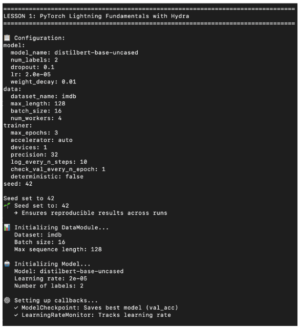
This is a major MLOps advantage because configuration-driven training allows experiments to be repeated, compared, and automated easily.

Viewing Logs and Metrics in TensorBoard

All training metrics are logged to:

logs/sentiment_classifier/

You can launch TensorBoard using:

$ tensorboard --logdir logs/

This screenshot shows how TensorBoard automatically tracks metrics (e.g., val_acc and val_loss) for each Hydra-versioned training run. Because the entire pipeline is configuration-driven, you can compare experiments side-by-side by smoothing curves, inspecting run histories, and validating that model performance trends remain consistent across seeds or hyperparameter overrides.

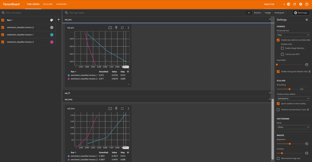
A typical figure here would show:

• Training vs. validation loss
• Validation accuracy
• Learning rate
• Iteration timeline

This screenshot reinforces that Lightning + TensorBoard gives you well-structured experiment tracking out of the box.

Where Checkpoints Are Saved

Lightning automatically saves your best checkpoint based on validation accuracy:

checkpoints/best-epoch=XX-val_acc=YY.ckpt

It also saves a last.ckpt for safety.

Lightning’s ModelCheckpoint callback saves the best-performing model (based on val_acc) and the final “last.ckpt” snapshot for safety. Because training is fully configuration-driven, each Hydra-run creates its own versioned checkpoint set, making it easy to resume, compare, or deploy models in a reproducible MLOps workflow.

This is often the moment readers see how cleanly Lightning organizes artifacts, which ties directly into the next DVC module.

Running Inference (Multiple Modes)

Once training completes, you can use the inference script in 3 different modes.

A) Single-Text Prediction

$ python src/inference.py --checkpoint "checkpoints/best-epoch=00-val_acc=0.8797.ckpt" --text "This movie was amazing!"

The screenshot shows the model being loaded from the selected checkpoint, the tokenizer initialization, and the final prediction with confidence for the given input text.

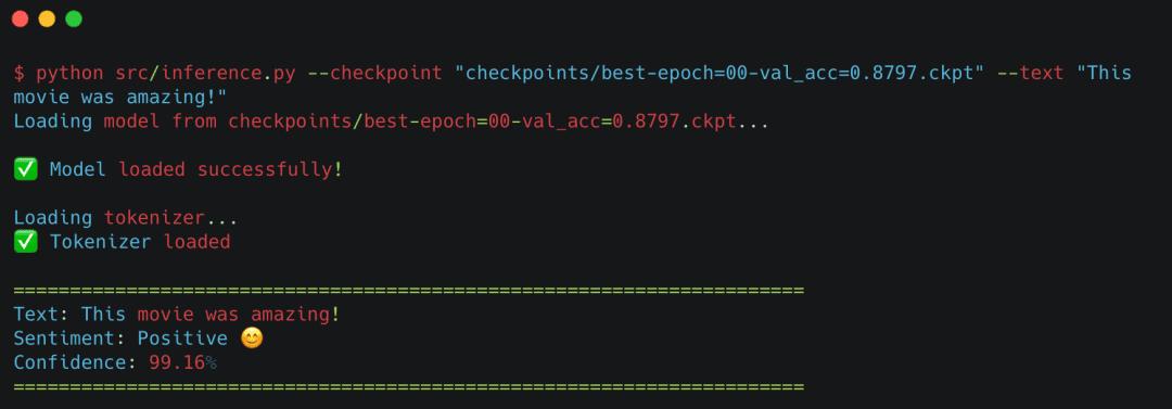
Lightning auto-loads the checkpoint, loads the tokenizer, moves tensors to the correct device, and returns a structured prediction.

B) Batch Inference from File

Create a file such as the following:

samples.txt
This movie was incredible.
The film was a disappointment.
I loved every character!

Then run:

$ python src/inference.py \
    --checkpoint checkpoints/best-epoch=*.ckpt \
    --input-file samples.txt

The screenshot shows the model loading, tokenizer initialization, per-review predictions with confidence scores, and a final summary of positive and negative counts. This demonstrates how the inference pipeline scales cleanly from single inputs to larger batches, which is a key requirement in practical MLOps workflows.

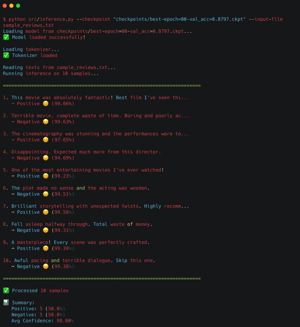
The script also prints a small summary (positive %, negative %, average confidence).

C) Interactive Mode

$ python src/inference.py \
    --checkpoint checkpoints/best-epoch=*.ckpt

You can then type reviews manually.

Figure 6 shows the interactive prompt, a sample user review (“The movie was good — just not great.”), and the model’s corresponding prediction with confidence. This mode is ideal for quick testing and showcasing the end-to-end inference flow after training your Lightning model.

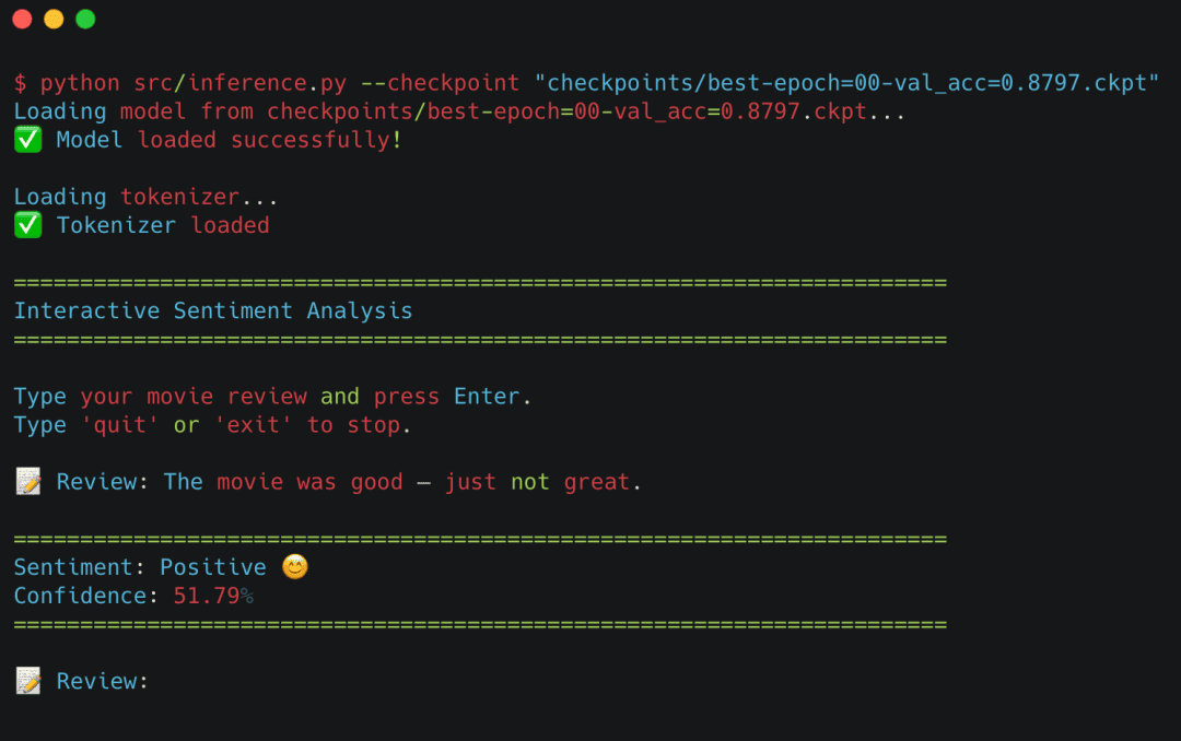
This mode is great for demos, lightweight testing, or API prototyping.

Device Auto-Selection (CPU, GPU, and MPS)

Your inference script includes this logic:

if device == "auto":
    device = "cuda" if torch.cuda.is_available() else "cpu"

When device is set to "auto", the script selects a CUDA-enabled graphics processing unit (GPU) if one is available. Otherwise, it selects the central processing unit (CPU). On Macs with Apple Silicon, you can also choose Metal Performance Shaders (MPS) explicitly by setting the device to "mps".

Lightning also handles device selection on the training side:

• If a GPU is available and the trainer is configured to use it, Lightning uses the GPU.
• If multiple GPUs are configured, Lightning uses DDP (Lesson 2).
• If no supported GPU is available, Lightning falls back to the CPU.

Figure 7 confirms that Lightning detected an MPS-capable GPU on macOS and will use it for training. It also reports that no Tensor Processing Unit (TPU) cores are available. This automation allows the training code to run across different hardware configurations without modification.

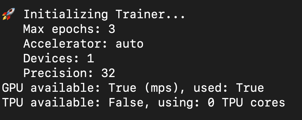
This flexibility dramatically improves developer experience (DX) because your code can run on any machine.

Summary: Why This Section Matters for MLOps

This “Run and Evaluate” section ties the entire workflow together:

• Hydra makes experiments repeatable and configurable.
• Lightning makes training structured and supports deterministic execution when configured appropriately.
• TensorBoard provides observability.
• Checkpoints preserve model state for downstream deployment.
• The inference script demonstrates end-to-end functionality.

This is precisely the level of workflow maturity expected in modern MLOps and LLMOps environments.

---

---

Summary

In this lesson, you learned how PyTorch Lightning and Hydra work together to bring structure, reproducibility, and MLOps-friendly practices to a modern NLP training pipeline. Instead of writing long, error-prone training loops, Lightning allowed you to organize your project into clean, isolated components: the LightningDataModule for handling all data operations and the LightningModule for model logic, optimization, and metrics. Hydra completed the picture by giving you a powerful configuration system that let you change hyperparameters, batch sizes, model choices, or even hardware strategies from the command line without touching a single line of Python.

You trained a sentiment classifier on the IMDB dataset using a fully modular workflow, ran experiments with different overrides, visualized metrics in TensorBoard, and saved reproducible checkpoints automatically. Most importantly, you saw how clean architecture and configuration-driven design make your training pipeline easier to extend, debug, monitor, and deploy. These capabilities are exactly what real-world MLOps demands.

In the next lesson, we will take this foundation and push it into production territory. You will learn how to scale the same codebase with distributed training (DDP and FSDP), mixed precision, and model export to ONNX and TorchScript, all while keeping the project structure identical. If you want to turn this into a robust, deployment-ready training workflow, just keep reading.

Citation Information

Singh, V. “Training with PyTorch Lightning: Structured MLOps Development,” PyImageSearch, S. Huot, A. Sharma, and P. Thakur, eds., 2026, https://pyimg.co/5fe4l

@incollection{Singh_2026_training-w-pytorch-lightning-structured-mlops-development,
  author = {Vikram Singh},
  title = {{Training with PyTorch Lightning: Structured MLOps Development}},
  booktitle = {PyImageSearch},
  editor = {Susan Huot and Aditya Sharma and Piyush Thakur},
  year = {2026},
  url = {https://pyimg.co/5fe4l},
}

To download the source code to this post (and be notified when future tutorials are published here on PyImageSearch), simply enter your email address in the form below!