Torch Hub Series #5: MiDaS — Model on Depth Estimation

In the previous part of this series, we discussed some state-of-the-art object detection models; YOLOv5 and SSD. In today’s tutorial, we will discuss MiDaS, an ingenious attempt to aid the depth estimation of images.

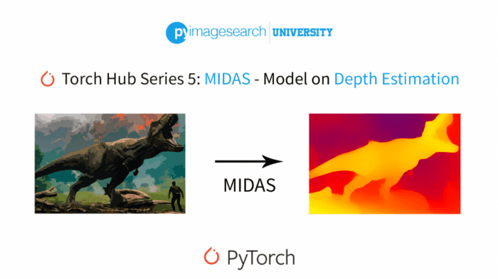
With this tutorial, we will create a basic intuition about the idea behind MiDaS and learn how to use it as a depth estimation inference tool.

This lesson is part 5 of a 6-part series on Torch Hub:

1. Torch Hub Series #1: Introduction to Torch Hub
2. Torch Hub Series #2: VGG and ResNet
3. Torch Hub Series #3: YOLO v5 and SSD — Models on Object Detection
4. Torch Hub Series #4: PGAN — Model on GAN
5. Torch Hub Series #5: MiDaS — Model on Depth Estimation (this tutorial)
6. Torch Hub Series #6: Image Segmentation

To learn how to use MiDaS on your custom data, just keep reading.

Torch Hub Series #5: MiDaS — Model on Depth Estimation

Introduction

First, let us understand what depth estimation is or why it is important. Depth estimation of an image predicts the order of objects (if the image was expanded in a 3D format) from the 2D image itself. It is an unequivocally difficult task since getting annotated data and datasets specializing in this area was a mammoth task itself. The use of depth estimation is far and wide, most noticeably in the domain of self-driving cars, where estimating the distance of objects around a car helps in navigation (Figure 1).

The researchers behind MiDaS have explained their motives in a very simple manner. They firmly assert that training models on a single dataset will not be robust when dealing with problem statements encompassing real-life issues. When models used in real-time are created, they should be robust enough to deal with as many situations and outliers as possible.

Keeping that in mind, the creators of MiDaS decided to train their model on multiple datasets. This includes datasets with different types of labels and objective functions. To achieve this, they devised a method to carry out computations in an appropriate output space compatible with all ground-truth representations.

The idea is very ingenious on paper, but the authors had to carefully devise loss functions and consider the challenges accompanying the choice of using multiple datasets. Since these datasets had different representations of depth estimation to varying degrees, an inherent scale ambiguity, and shift ambiguity come up, as the paper’s authors addressed.

Now, since the datasets in all probability would follow distributions different from each other. Hence the issues are pretty much expected. However, the authors propose solutions to each of the challenges. The end product was a robust depth estimator, which was as efficient as accurate. In Figure 2, we see some results shown in the paper.

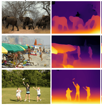
The idea of cross dataset learning isn’t new, but the complications that arise from getting the ground truths to a common output space are extremely tough to get by. However, the paper explains each step extensively, starting with the intuition right to the mathematical definition of the losses used.

Let’s see how we can use the MiDaS model to find the inverse depth of our custom images.

Configuring Your Development Environment

To follow this guide, you need to have the OpenCV library installed on your system.

Luckily, OpenCV is pip-installable:

$ pip install opencv-contrib-python

If you need help configuring your development environment for OpenCV, I highly recommend that you read my pip install OpenCV guide — it will have you up and running in a matter of minutes.

Having Problems Configuring Your Development Environment?

All that said, are you:

• Short on time?
• Learning on your employer’s administratively locked system?
• Wanting to skip the hassle of fighting with the command line, package managers, and virtual environments?
• Ready to run the code right now on your Windows, macOS, or Linux system?

Then join PyImageSearch University today!

Gain access to Jupyter Notebooks for this tutorial and other PyImageSearch guides that are pre-configured to run on Google Colab’s ecosystem right in your web browser! No installation required.

And best of all, these Jupyter Notebooks will run on Windows, macOS, and Linux!

Project Structure

We first need to review our project directory structure.

Start by accessing the “Downloads” section of this tutorial to retrieve the source code and example images.

From there, take a look at the directory structure:

!tree .
.
├── midas_inference.py
├── output
│   └── midas_output
│       └── output.png
└── pyimagesearch
    ├── config.py
    └── data_utils.py

Inside the pyimagesearch directory, we have 2 scripts:

• config.py: Contains an end to end configuration pipeline for the project
• data_utils.py: Houses the two data utility functions we’ll be using in the project

In the parent directory, we have one single script:

• midas_inference.py: To infer from the pretrained MiDaS model

Finally, we have the output directory, which will house the result plots obtained from running the script.

Downloading the Dataset

Owing to its compactness, we’ll be using the Dogs & Cats Images dataset from Kaggle again.

$ mkdir ~/.kaggle
$ cp <path to your kaggle.json> ~/.kaggle/
$ chmod 600 ~/.kaggle/kaggle.json
$ kaggle datasets download -d chetankv/dogs-cats-images
$ unzip -qq dogs-cats-images.zip
$ rm -rf "/content/dog vs cat"

As explained in previous posts of this series, you’ll need your own unique kaggle.json file to connect to the Kaggle API (Line 2). The chmod 600 command on Line 3 will allow your script complete access to read and write files.

The following kaggle datasets download command (Line 4) allows you to download any dataset hosted on their website. Finally, we have the unzip command and an auxiliary delete command for the unnecessary additions (Lines 5 and 6).

Let’s move on to the configuration pipeline.

Configuring the Prerequisites

Inside the pyimagesearch directory, you’ll find a script called config.py. This script will house the complete end-to-end configuration pipeline of our project.

# import the necessary packages
import torch
import os

# define the root directory followed by the test dataset paths
BASE_PATH = "dataset"
TEST_PATH = os.path.join(BASE_PATH, "test_set")

# specify image size and batch size
IMAGE_SIZE = 384
PRED_BATCH_SIZE = 4

# determine the device type 
DEVICE = torch.device("cuda") if torch.cuda.is_available() else "cpu"

# define paths to save output 
OUTPUT_PATH = "output"
MIDAS_OUTPUT = os.path.join(OUTPUT_PATH, "midas_output")

First, we have the BASE_PATH variable as a pointer to the dataset directory (Line 6). We’re not doing any additional tinkering to our models, so we’ll only use the test set (Line 7).

On Line 10, we have a variable named IMAGE_SIZE, set to 384, as a mandate for our MiDaS model input. The prediction batch size is set to 4 (Line 11), but readers are encouraged to play around with different sizes.

It’s advisable that you have a CUDA-compatible device for today’s project (Line 14), but since we’re not going for any heavy training, CPUs should work fine too.

Lastly, we have created paths to save the outputs obtained from the model inferences (Lines 17 and 18).

We’ll only be using a single helper function to aid our pipeline in today’s task. For that, we’ll move onto the second script in the pyimagesearch directory, data_utils.py.

# import the necessary packages
from torch.utils.data import DataLoader

def get_dataloader(dataset, batchSize, shuffle=True):
	# create a dataloader and return it
	dataLoader= DataLoader(dataset, batch_size=batchSize,
		shuffle=shuffle)
	return dataLoader

On Line 4, we have the get_dataloader function, which takes in the dataset, batch size, and shuffle variables as its arguments. This function returns a generator like the PyTorch Dataloader instance which will help us deal with huge data (Line 6).

That concludes our utilities. Let’s move on to the inference script.

Finding Inverse Depth Estimation Using MiDaS

At this time, a very logical question might pop up in your mind; Why are we going to such lengths to get inference on a handful of images?

The path we have chosen here is a full-proof way of dealing with huge datasets, and the pipeline will be useful even if you choose to train the model for fine-tuning later down the road. We have also considered preparing the data as best we can without invoking the premade functions of the MiDaS repository.

# import necessary packages
from pyimagesearch.data_utils import get_dataloader
from pyimagesearch import config
from torchvision.transforms import Compose, ToTensor, Resize
from torchvision.datasets import ImageFolder
import matplotlib.pyplot as plt
import torch
import os

# create the test dataset with a test transform pipeline and
# initialize the test data loader
testTransform = Compose([
	Resize((config.IMAGE_SIZE, config.IMAGE_SIZE)), ToTensor()])
testDataset = ImageFolder(config.TEST_PATH, testTransform)
testLoader = get_dataloader(testDataset, config.PRED_BATCH_SIZE)

As mentioned earlier, since we will be only using the test set, we have created a PyTorch test transform instance where we are reshaping the images and converting them to tensors (Lines 12 and 13).

If your dataset is in the format as the one we are using for our project (i.e., images under the folder named as labels), then we can use the ImageFolder function to create a PyTorch Dataset instance (Line 14). Lastly, we use the previously defined get_dataloader function to generate a Dataloader instance (Line 15).

# initialize the midas model using torch hub
modelType = "DPT_Large" 
midas = torch.hub.load("intel-isl/MiDaS", modelType)

# flash the model to the device and set it to eval mode
midas.to(device)
midas.eval()

Next, we use the torch.hub.load function to load the MiDaS model in our local runtime (Lines 18 and 19). Again, several available choices can be called here, all of which can be found here. Finally, we load the model to our device and set it to evaluation mode (Lines 22 and 23).

# initialize iterable variable
sweeper = iter(testLoader)

# grab a batch of test data send the images to the device
print("[INFO] getting the test data...")
batch = next(sweeper)
(images, _) = (batch[0], batch[1])
images = images.to(config.DEVICE) 
 
# turn off auto grad
with torch.no_grad():
	# get predictions from input
	prediction = midas(images)

	# unsqueeze the predictions batchwise
	prediction = torch.nn.functional.interpolate(
		prediction.unsqueeze(1), size=[384,384], mode="bicubic",
		align_corners=False).squeeze()

# store the predictions in a numpy array
output = prediction.cpu().numpy()

The sweeper variable on Line 26 will act as the iterable variable of the testLoader. Each time we run the command on Line 30, we’ll get a new batch of data from the testLoader. On Line 31, we unpack the batch into images and labels, keeping only the images.

After loading the images to our device (Line 32), we turn off automatic gradients and pass the images through the model (Lines 35-37). On Line 40, we use a beautiful utility function called torch.nn.functional.interpolate to unpack our predictions into a valid 3-channel image format.

Finally, we store the reformatted predictions to an output variable in numpy format (Line 45).

# define row and column variables
rows = config.PRED_BATCH_SIZE
cols = 2

# define axes for subplots
axes = []
fig=plt.figure(figsize=(10, 20))

# loop over the rows and columns
for totalRange in range(rows*cols):
	axes.append(fig.add_subplot(rows, cols, totalRange+1))

	# set up conditions for side by side plotting 
	# of ground truth and predictions
	if totalRange % 2 == 0:
		plt.imshow(images[totalRange//2]
			.permute((1, 2, 0)).cpu().detach().numpy())
	else :
		plt.imshow(output[totalRange//2])
fig.tight_layout()

# build the midas output directory if not already present
if not os.path.exists(config.MIDAS_OUTPUT):
	os.makedirs(config.MIDAS_OUTPUT)

# save plots to output directory
print("[INFO] saving the inference...")
outputFileName = os.path.join(config.MIDAS_OUTPUT, "output.png")
plt.savefig(outputFileName)

To plot our results, we first define the rows and column variables to define the grid format (Lines 48 and 49). On Lines 52 and 53, we define the subplot list and figure size.

Looping over the rows and columns, we define a methodology where the inverse depth estimation and the ground truth images get plotted side by side (Lines 56-66).

Lastly, we save the figure to our desired path (Lines 69 and 75).

With our inference script done, let’s check out some of the results.

MiDaS Inference Results

Most of the images in our dataset will have either a cat or dog in the forefront. There might not be enough images with background, but the MiDaS model should give us an output that depicts the cat or dog in the foreground decisively. That is exactly what has happened in our inference images ( Figures 4-7).

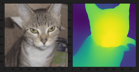
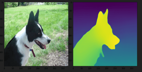
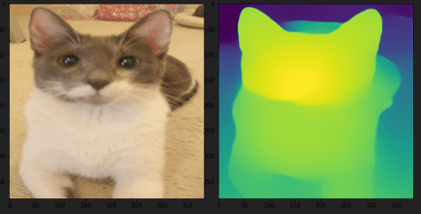
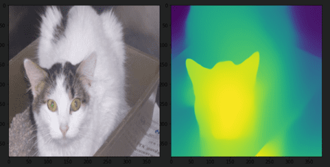
Although the spectacular capabilities of MiDaS can be seen in all the inference images, we can look into each of them in-depth and draw out some more observations.

In Figure 4, not only is the cat depicted in the foreground, but its head is closer to the camera than its body (shown by the change in color). In Figure 5, since the field mainly covers the image, there is a clear distinction between the dog and the field. In both Figure 6 and Figure 7, the cat’s head is depicted closer than its body.

Summary

Grasping the importance of MiDaS in today’s world is an important step for us. Imagine how much help a perfect depth estimator would be for autonomous vehicles. Since autonomous cars almost completely depend on utilities like LiDAR (light detection and ranging), cameras, SONAR (sound navigation and ranging), etc., having a full-proof system of depth estimation of its surroundings will make travel safer and take the load off the other sensor systems.

The second most important thing to note about MiDaS is the usage of cross dataset mixing. While it has recently gained momentum, executing it to perfection takes considerable time and planning. Moreover, MiDaS does this on a domain that significantly impacts a real-world issue.

I hope this tutorial served as a gateway to pique your interest regarding all things about autonomous systems and depth estimation. Feel free to try this out with your custom datasets and share the results.

Citation Information

Chakraborty, D. “Torch Hub Series #5: MiDaS — Model on Depth Estimation,” PyImageSearch, 2022, https://pyimagesearch.com/2022/01/17/torch-hub-series-5-midas-model-on-depth-estimation/

@article{Chakraborty_2022_THS5,
  author = {Devjyoti Chakraborty},
  title = {Torch Hub Series \#5: {MiDaS} — Model on Depth Estimation},
  journal = {PyImageSearch},
  year = {2022},
  note = {https://pyimagesearch.com/2022/01/17/torch-hub-series-5-midas-model-on-depth-estimation/},
}

To download the source code to this post (and be notified when future tutorials are published here on PyImageSearch), simply enter your email address in the form below!